Toolkit for analysis and identification of hematological cell types from heterogeneous single cell RNA-seq data

Project description
Digital Cell Sorter


Identification of hematological cell types from heterogeneous single cell RNA-seq data.
Polled Digital Cell Sorter (p-DCS): Automatic identification of hematological cell types from single cell RNA-sequencing clusters Sergii Domanskyi, Anthony Szedlak, Nathaniel T Hawkins, Jiayin Wang, Giovanni Paternostro & Carlo Piermarocchi, BMC Bioinformatics volume 20, Article number: 369 (2019)
The documentation is available at https://digital-cell-sorter.readthedocs.io/.
Getting Started
These instructions will get you a copy of the project up and running on your machine for data analysis, development or testing purposes.
Prerequisites
The code runs in Python >= 3.7 environment.
It is highly recommended to install Anaconda. Installers are available at https://www.anaconda.com/distribution/
It uses packages numpy, pandas, matplotlib, scikit-learn, scipy,
mygene, fftw, pynndescent, networkx, python-louvain, fitsne
and a few other standard Python packages. Most of these packages are installed with installation of the
latest release of DigitalCellSorter:
pip install DigitalCellSorter
Alternatively, you can install this module directly from GitHub using:
pip install git+https://github.com/sdomanskyi/DigitalCellSorter
Also one can create a local copy of this project for development purposes by running:
git clone https://github.com/sdomanskyi/DigitalCellSorter
To install fftw from the conda-forge channel add conda-forge to your channels.
Once the conda-forge channel has been enabled, fftw can be installed as follows:
conda config --add channels conda-forge
conda install fftw
Loading the package
In your script import the package:
import DigitalCellSorter
Create an instance of class DigitalCellSorter. Here, for simplicity, we use Default parameter values:
DCS = DigitalCellSorter.DigitalCellSorter()
During the initialization the following parameters can be specified (click me)
dataName: name used in output files, Default ''
geneListFileName: marker cell type list name, Default None
mitochondrialGenes: list of mitochondrial genes for quality conrol routine, Default None
sigmaOverMeanSigma: threshold to consider a gene constant, Default 0.3
nClusters: number of clusters, Default 5
nComponentsPCA: number of pca components, Default 100
nSamplesDistribution: number of random samples to generate, Default 10000
saveDir: directory for output files, Default is current directory
makeMarkerSubplots: whether to make subplots on markers, Default True
makePlots: whether to make all major plots, Default True
votingScheme: voting shceme to use instead of the built-in, Default None
availableCPUsCount: number of CPUs available, Default os.cpu_count()
zScoreCutoff: zscore cutoff when calculating Z_mc, Default 0.3
clusterName: parameter used in subclustering, Default None
doQualityControl: whether to remove low quality cells, Default True
doBatchCorrection: whether to correct data for batches, Default False
These and other parameters can be modified after initialization using, e.g.:
DCS.toggleMakeStackedBarplot = False
Gene Expression Data Format
The input gene expression data is expected in one of the following formats:
- Spreadsheet of comma-separated values
csvcontaining condensed matrix in a form('cell', 'gene', 'expr'). If there are batches in the data the matrix has to be of the form('batch', 'cell', 'gene', 'expr'). Columns order can be arbitrary.
Examples:
| cell | gene | expr |
|---|---|---|
| C1 | G1 | 3 |
| C1 | G2 | 2 |
| C1 | G3 | 1 |
| C2 | G1 | 1 |
| C2 | G4 | 5 |
| ... | ... | ... |
or:
| batch | cell | gene | expr |
|---|---|---|---|
| batch0 | C1 | G1 | 3 |
| batch0 | C1 | G2 | 2 |
| batch0 | C1 | G3 | 1 |
| batch1 | C2 | G1 | 1 |
| batch1 | C2 | G4 | 5 |
| ... | ... | ... | ... |
- Spreadsheet of comma-separated values
csvwhere rows are genes, columns are cells with gene expression counts. If there are batches in the data the spreadsheet the first row should be'batch'and the second'cell'.
Examples:
| cell | C1 | C2 | C3 | C4 |
|---|---|---|---|---|
| G1 | 3 | 1 | 7 | |
| G2 | 2 | 2 | 2 | |
| G3 | 3 | 1 | 5 | |
| G4 | 10 | 5 | 4 | |
| ... | ... | ... | ... | ... |
or:
| batch | batch0 | batch0 | batch1 | batch1 |
|---|---|---|---|---|
| cell | C1 | C2 | C3 | C4 |
| G1 | 3 | 1 | 7 | |
| G2 | 2 | 2 | 2 | |
| G3 | 3 | 1 | 5 | |
| G4 | 10 | 5 | 4 | |
| ... | ... | ... | ... | ... |
Pandas DataFramewhereaxis 0is genes andaxis 1are cells. If the are batched in the data then the index ofaxis 1should have two levels, e.g.('batch', 'cell'), with the first level indicating patient, batch or expreriment where that cell was sequenced, and the second level containing cell barcodes for identification.
Examples:
df = pd.DataFrame(data=[[2,np.nan],[3,8],[3,5],[np.nan,1]],
                  index=['G1','G2','G3','G4'],
                  columns=pd.MultiIndex.from_arrays([['batch0','batch1'],['C1','C2']], names=['batch', 'cell']))
Pandas Serieswhere index should have two levels, e.g.('cell', 'gene'). If there are batched in the data the first level should be indicating patient, batch or expreriment where that cell was sequenced, the second level cell barcodes for identification and the third level gene names.
Examples:
se = pd.Series(data=[1,8,3,5,5],
               index=pd.MultiIndex.from_arrays([['batch0','batch0','batch1','batch1','batch1'],
                                                ['C1','C1','C1','C2','C2'],
                                                ['G1','G2','G3','G1','G4']], names=['batch', 'cell', 'gene']))
Any of the data types outlined above need to be prepared/validated with a function prepare().
Let us demonstrate this on the input of type 1:
df_expr = DCS.prepare('data/testData/dataFileCondensedWithBatches.tsv')
Other Data
markersDCS.xlsx: An excel book with marker data. Rows are markers and columns are cell types.
'1' means that the gene is a marker for that cell type, and '0' otherwise.
This gene marker file included in the package is used by Default.
If you use your own file it has to be prepared in the same format (including the two-line header). Note that only the first worksheet will be read,
and its name can be arbitrary. The first column should contain gene names. The second row should contain cell types, and the first row how
those cell types are grouped. If any of the cell types need to be skipped, have "NA" in the corresponding cell of the first row of that cell type.
See example below:
| A | B | C | D | E | F | G | H | I | J | K | L | M | ... |
|---|---|---|---|---|---|---|---|---|---|---|---|---|---|
| B cells | B cells | B cells | T cells | T cells | T cells | T cells | T cells | T cells | T cells | NK cells | NK cells | ... | |
| Marker | B cells naive | B cells memory | Plasma cells | T cells CD8 | T cells CD4 naive | T cells CD4 memory resting | T cells CD4 memory activated | T cells follicular helper | T cells regulatory (Tregs) | T cells gamma delta | NK cells resting | NK cells activated | ... |
| ABCB4 | 1 | 0 | 0 | 0 | 0 | 0 | 0 | 0 | 0 | 0 | 0 | 0 | ... |
| ABCB9 | 0 | 0 | 1 | 0 | 0 | 0 | 0 | 0 | 0 | 0 | 0 | 0 | ... |
| ACAP1 | 0 | 0 | 0 | 0 | 1 | 0 | 0 | 0 | 0 | 0 | 0 | 0 | ... |
| ACHE | 0 | 0 | 0 | 0 | 0 | 0 | 0 | 0 | 0 | 0 | 0 | 0 | ... |
| ACP5 | 0 | 0 | 0 | 0 | 0 | 0 | 0 | 0 | 0 | 0 | 0 | 0 | ... |
| ADAM28 | 1 | 1 | 0 | 0 | 0 | 0 | 0 | 0 | 0 | 0 | 0 | 0 | ... |
| ADAMDEC1 | 0 | 0 | 0 | 0 | 0 | 0 | 0 | 0 | 0 | 0 | 0 | 0 | ... |
| ADAMTS3 | 0 | 0 | 0 | 0 | 0 | 0 | 0 | 0 | 0 | 0 | 0 | 0 | ... |
| ADRB2 | 0 | 0 | 0 | 0 | 0 | 0 | 0 | 0 | 0 | 0 | 0 | 0 | ... |
| AIF1 | 0 | 0 | 0 | 0 | 0 | 0 | 0 | 0 | 0 | 0 | 0 | 0 | ... |
| AIM2 | 0 | 1 | 0 | 0 | 0 | 0 | 0 | 0 | 0 | 0 | 0 | 0 | ... |
| ALOX15 | 0 | 0 | 0 | 0 | 0 | 0 | 0 | 0 | 0 | 0 | 0 | 0 | ... |
| ALOX5 | 0 | 1 | 0 | 0 | 0 | 0 | 0 | 0 | 0 | 0 | 0 | 0 | ... |
| AMPD1 | 0 | 0 | 1 | 0 | 0 | 0 | 0 | 0 | 0 | 0 | 0 | 0 | ... |
| ANGPT4 | 0 | 0 | 1 | 0 | 0 | 0 | 0 | 0 | 0 | 0 | 0 | 0 | ... |
| ... | ... | ... | ... | ... | ... | ... | ... | ... | ... | ... | ... | ... | ... |
Human.MitoCarta2.0.csv: An csv spreadsheet with human mitochondrial genes, created within work
MitoCarta2.0: an updated inventory of mammalian mitochondrial proteins
Sarah E. Calvo, Karl R. Clauser, Vamsi K. Mootha, Nucleic Acids Research, Volume 44, Issue D1, 4 January 2016, Pages D1251–D1257.
Functionality
Overall
The main class for cell sorting functions and producing output images is DigitalCellSorter
The class includes tools for:
-
Pre-preprocessing of single cell mRNA sequencing data (gene expression data)
- Cleaning: filling in missing values, zemoving all-zero genes and cells, converting gene index to a desired convention, etc.
- Normalizing: rescaling all cells expression, log-transforming, etc.
-
Quality control
-
Batch effects correction
-
Cells anomaly score evaluation
-
Dimensionality reduction
-
Clustering (Hierarchical, K-Means, knn-graph-based, etc.)
-
Annotating cell types
-
Vizualization
- t-SNE layout plot
- Quality Control histogram plot
- Marker expression t-SNE subplot
- Marker-centroids expression plot
- Voting results matrix plot
- Cell types stacked barplot
- Anomaly scores plot
- Histogram null distribution plot
- New markers plot
- Sankey diagram (a.k.a. river plot)
-
Post-processing functions, e.g. extract cells of interest, find significantly expressed genes, plot marker expression of the cells of interest, etc.
Visualization
Function visualize() or process() will produce all necessary files for post-analysis of the data.
The visualization tools include:
makeMarkerExpressionPlot(): a heatmap that shows all markers and their expression levels in the clusters, in addition this figure contains relative (%) and absolute (cell counts) cluster sizes

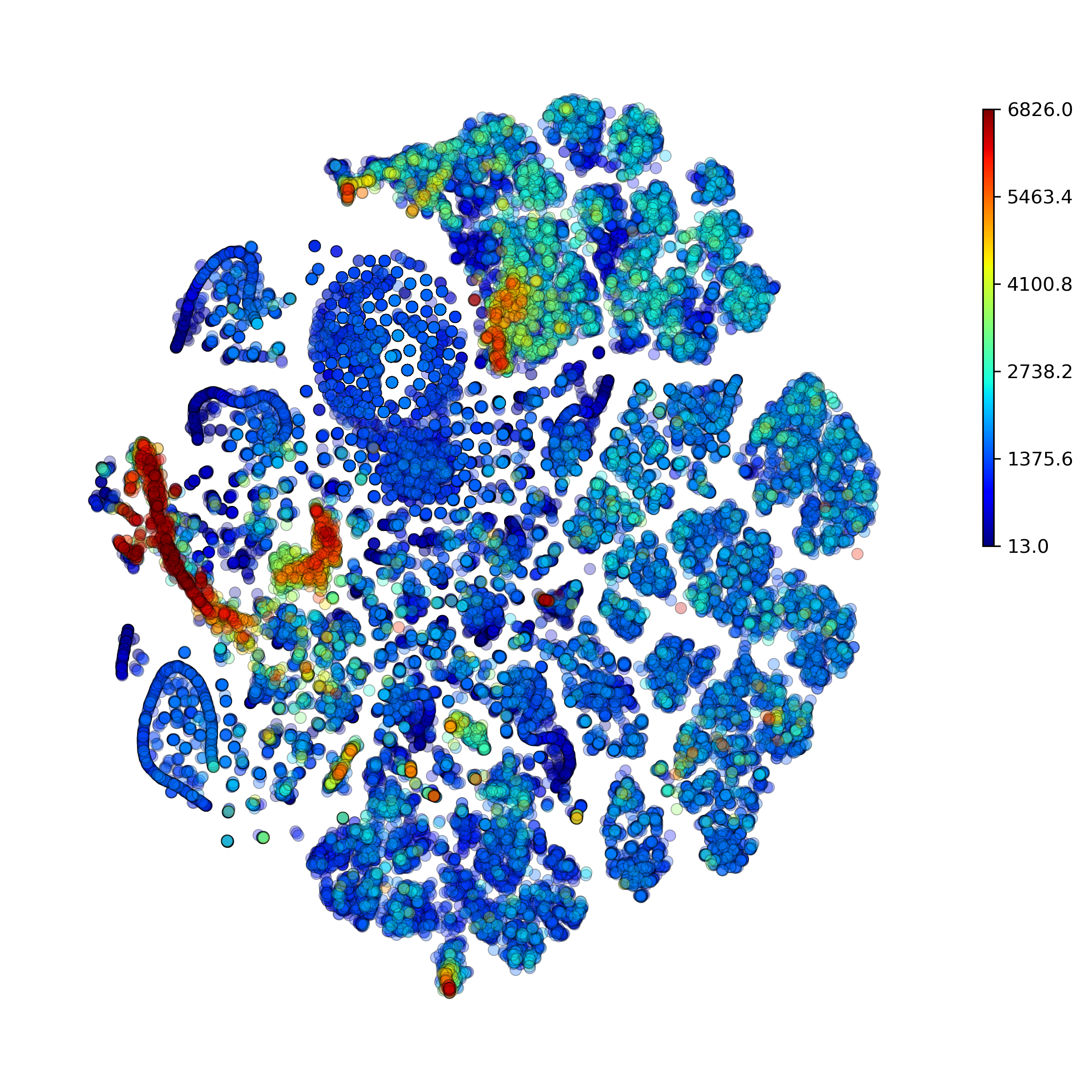
getIndividualGeneExpressionPlot(): t-SNE layout colored by individual gene's expression

makeVotingResultsMatrixPlot(): z-scores of the voting results for each input cell type and each cluster, in addition this figure contains relative (%) and absolute (cell counts) cluster sizes

makeHistogramNullDistributionPlot(): null distribution for each cluster and each cell type illustrating the "machinery" of the Digital Cell Sorter
makeQualityControlHistogramPlot(): Quality control histogram plots
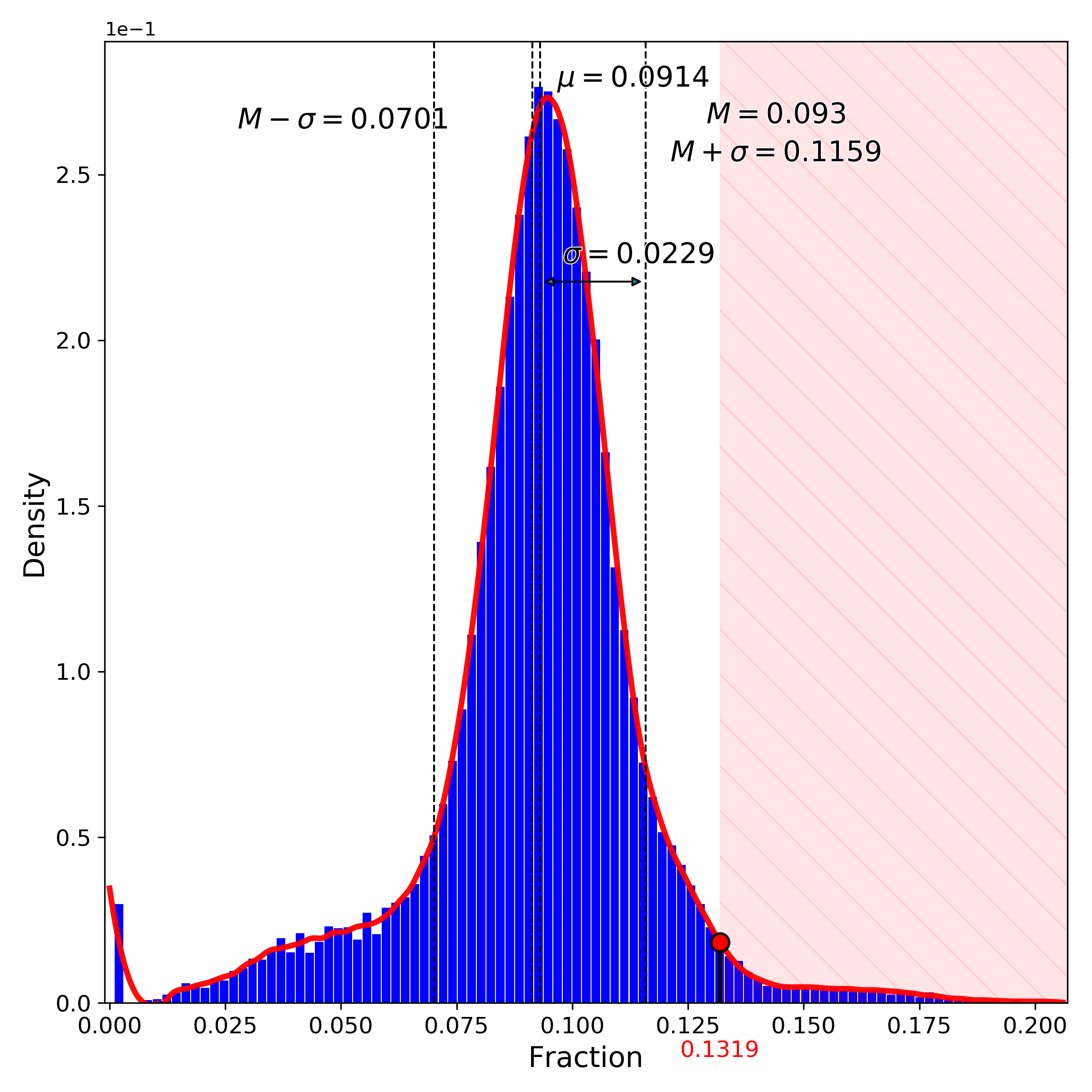
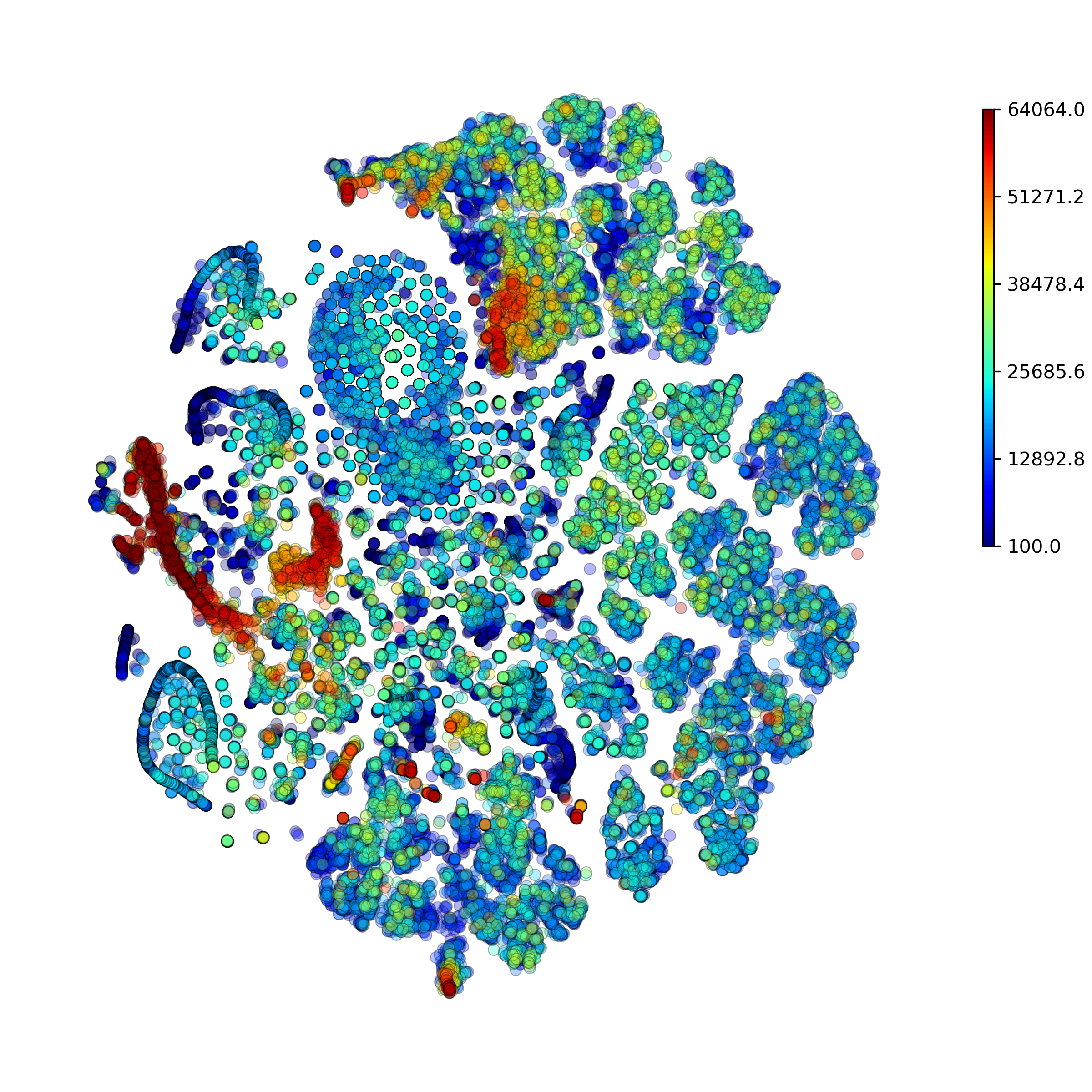
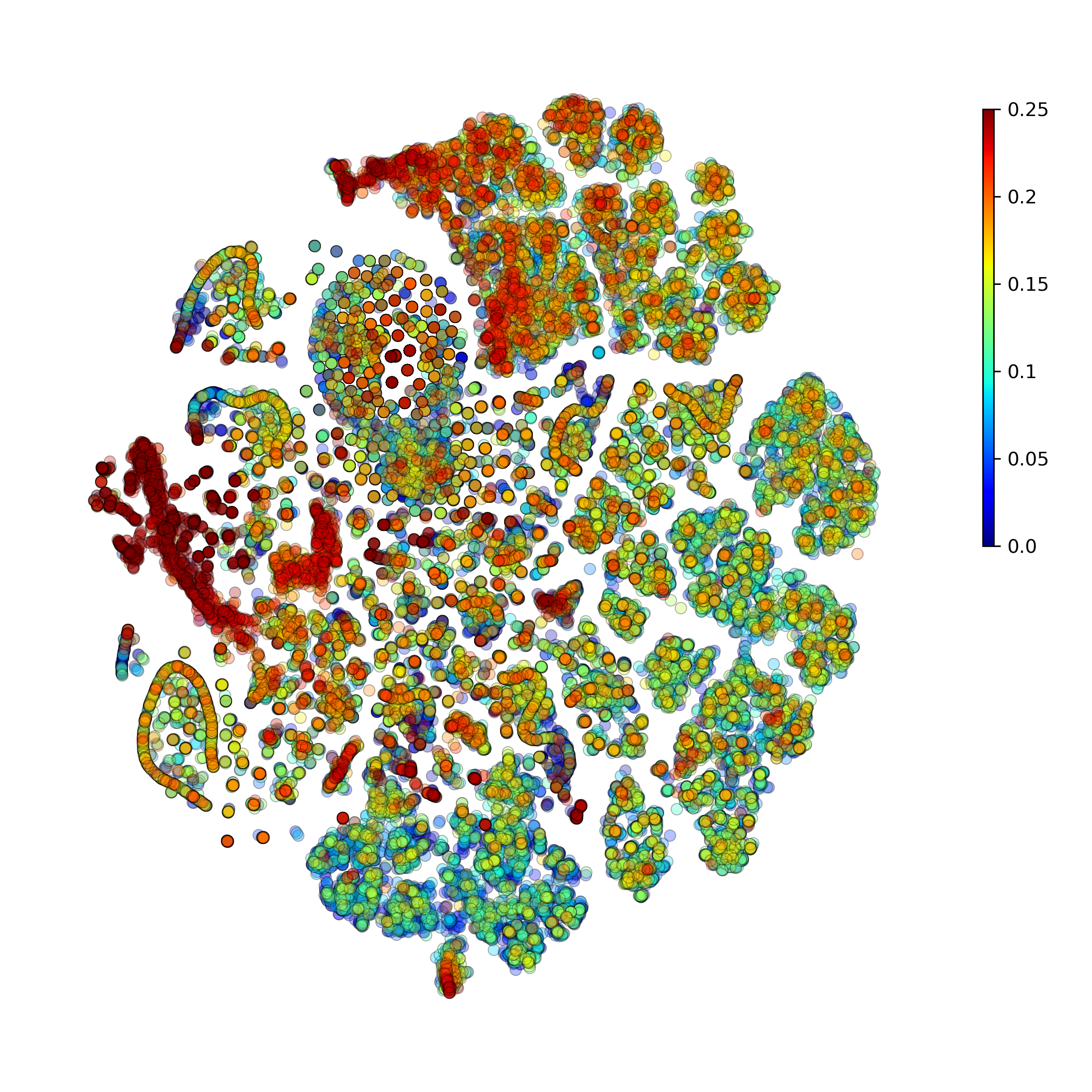
makeTSNEplot(): t-SNE layouts colored by number of unique genes expressed, number of counts measured, and a faraction of mitochondrial genes..
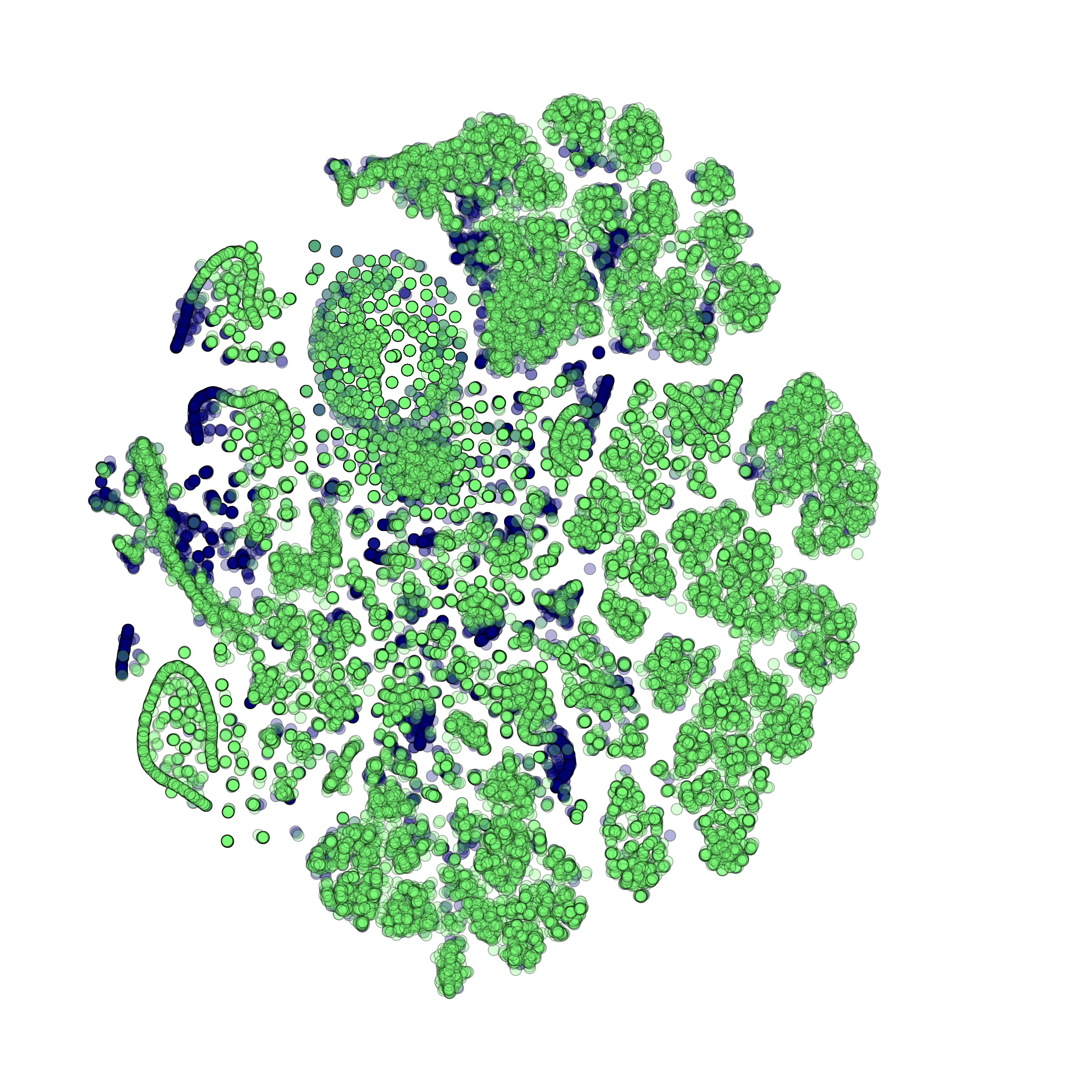
Effect of batch correction demostrated on combining BM1, BM2, BM3 and processing the data jointly without (left) and with (right) batch correction option:


makeStackedBarplot(): plot with fractions of various cell types

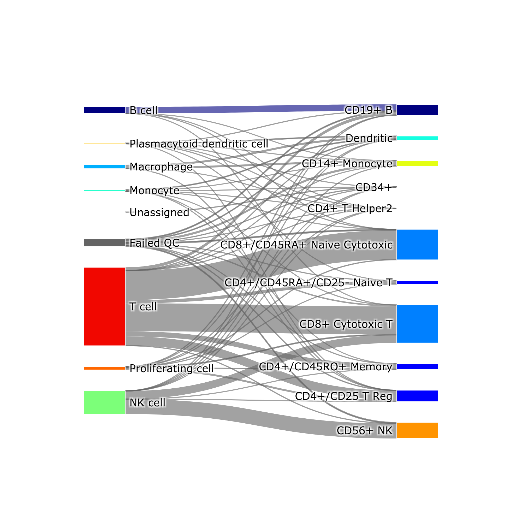
makeSankeyDiagram(): river plot to compare various results
(see interactive HTML version, download it and open in a browser)
getAnomalyScoresPlot(): plot with anomaly scores per cell

Calculate and plot anomaly scores for an arbitrary cell type or cluster:


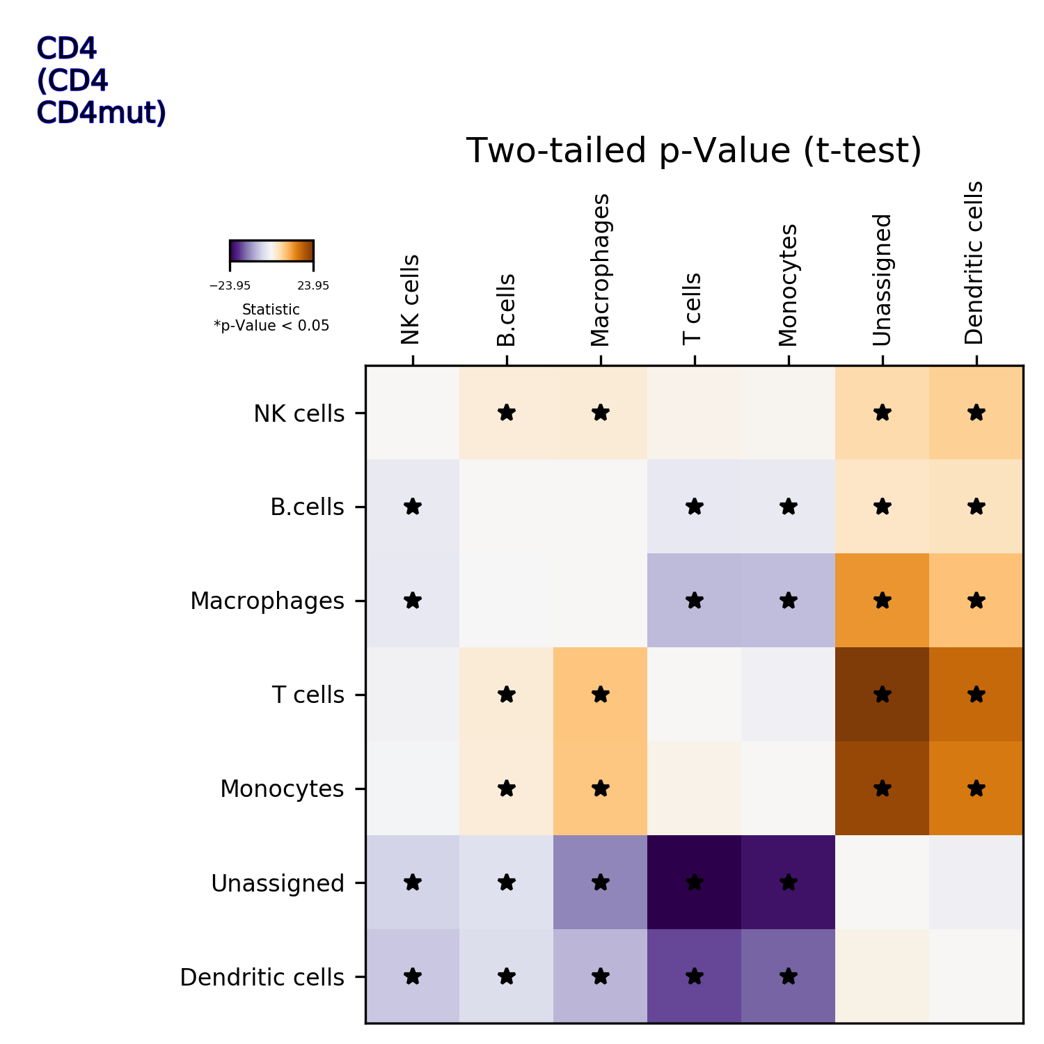
getIndividualGeneTtestPlot(): Produce heatmap plot of t-test p-Values calculated gene-pair-wise from the annotated clusters
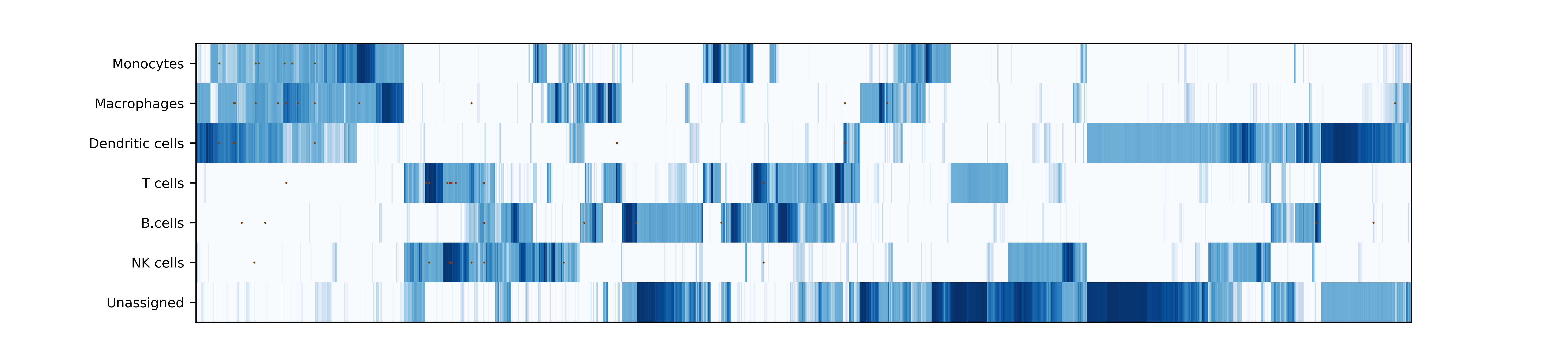
makePlotOfNewMarkers(): genes significantly expressed in the annotated cell types
Demo
Usage
We have made an example execution file demo.py that shows how to use DigitalCellSorter.
In the demo, folder data is intentionally left empty. The reader can download the file ica_bone_marrow_h5.h5
from https://preview.data.humancellatlas.org/ (Raw Counts Matrix - Bone Marrow) and place in folder data.
The file is ~485Mb and contains all 378000 cells from 8 bone marrow donors (BM1-BM8).
In our example, the data of BM1 is prepared by
function PrepareDataOnePatient() in module ReadPrepareDataHCApreviewDataset.
Load this function, and call it to create a BM1.h5 file (HDF file of input type 3) in the data folder:
from DigitalCellSorter.ReadPrepareDataHCApreviewDataset import PrepareDataOnePatient
PrepareDataOnePatient(os.path.join('data', 'ica_bone_marrow_h5.h5'), 'BM1', os.path.join('data', ''))
Main cell types
In these instructions we have already created an instance of DigitalCellSorter class (see section Loading the package) .
Let's modify some of the DCS attributes:
DCS.dataName = 'BM1'
DCS.saveDir = os.path.join(os.path.dirname(__file__), 'output', 'BM1', '')
DCS.nClusters = 20
Now we are ready to load the data, prepare(validate) it and process. The function process()
takes takes as an input parameter a pandas DataFrame validated by function prepare():
df_expr = pd.read_hdf(os.path.join('data', 'BM1.h5'), key='BM1', mode='r')
df_expr = DCS.prepare(df_expr)
DCS.process(df_expr)
This will launch the processing workflow detailed in our paper and generate the plots. If you don't need any plots and
looking forward to use post-processing tools, call function process() with an additional parameter:
DCS.process(df_expr, visualize=False)
Then, if necessary, you can generate all the default plots by:
DCS.visualize()
Cell sub-types
Further analysis can be done on cell types of interest, e.g. here 'T cell' and 'B cell'. Let's create a new instance of DigitalCellSorter to run "sub-analysis" with it:
DCSsub = DigitalCellSorter.DigitalCellSorter(dataName=DCS.dataName,
                                            nClusters=10,
                                            doQualityControl=False)
It is important to disable Quality control, because the low quality cells have already been identified and filtered with DCS.
Also dataName parameter points to the location processed with DCS.
Next modify a few other attributes and process cell type 'T cell':
DCSsub.subclusteringName = 'T cell'
DCSsub.saveDir = os.path.join(os.path.dirname(__file__), 'output', DCS.dataName, 'subclustering T cell', '')
DCSsub.geneListFileName = os.path.join(os.path.dirname(__file__), 'docs', 'examples', 'CIBERSORT_T_SUB.xlsx')

DCSsub.process(df_expr[DCS.getCells(celltype='T cell')])
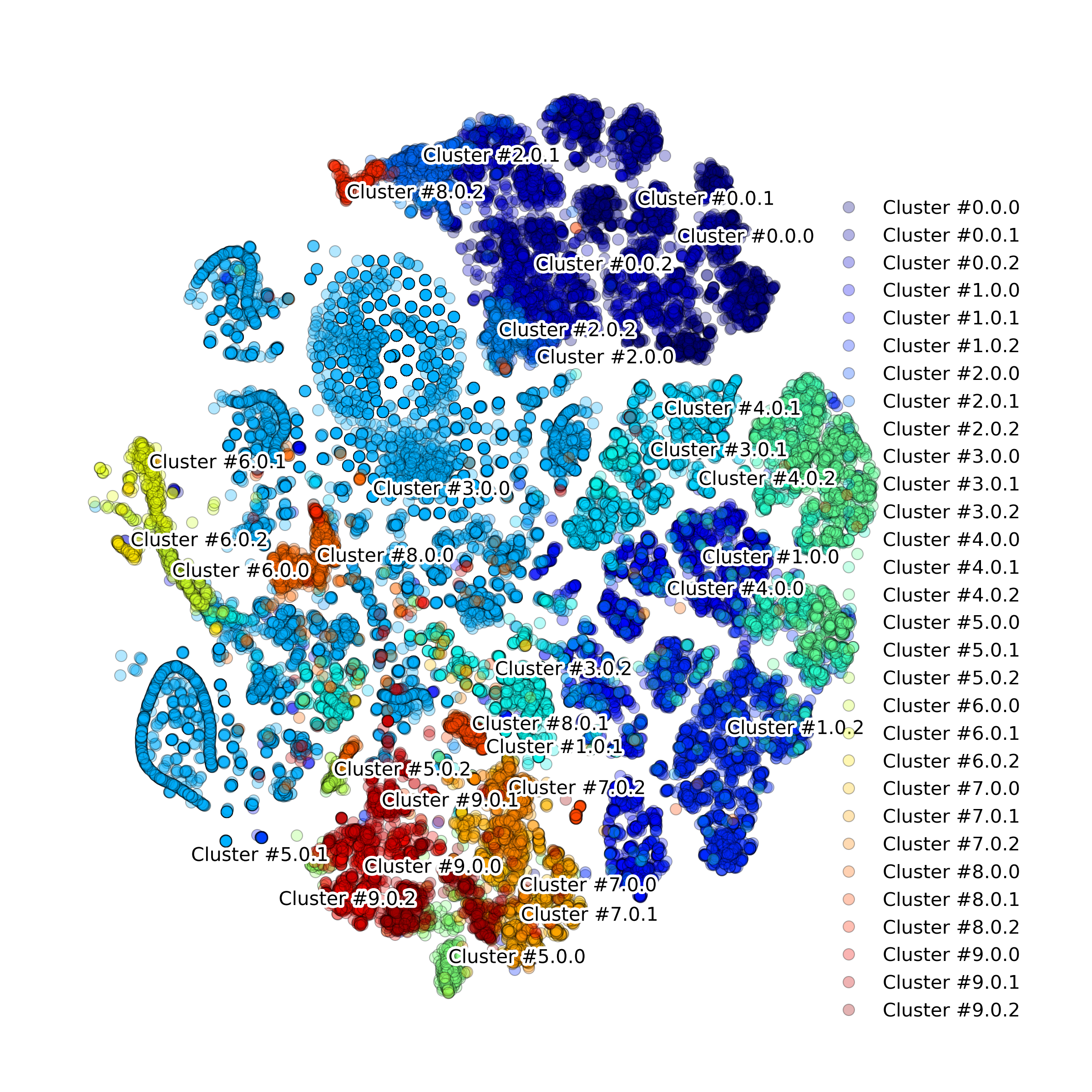
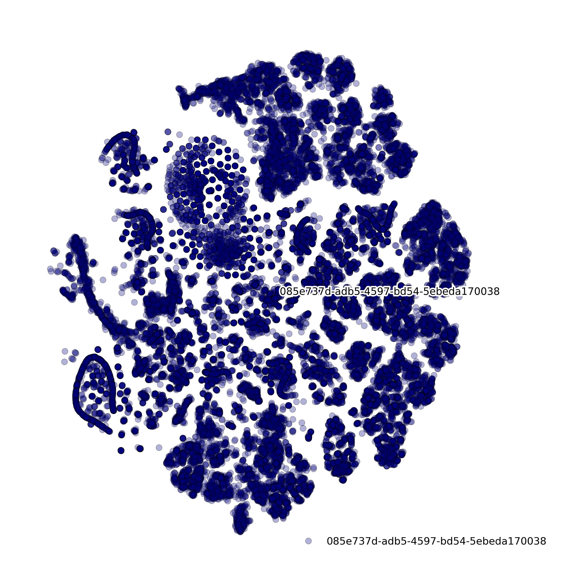
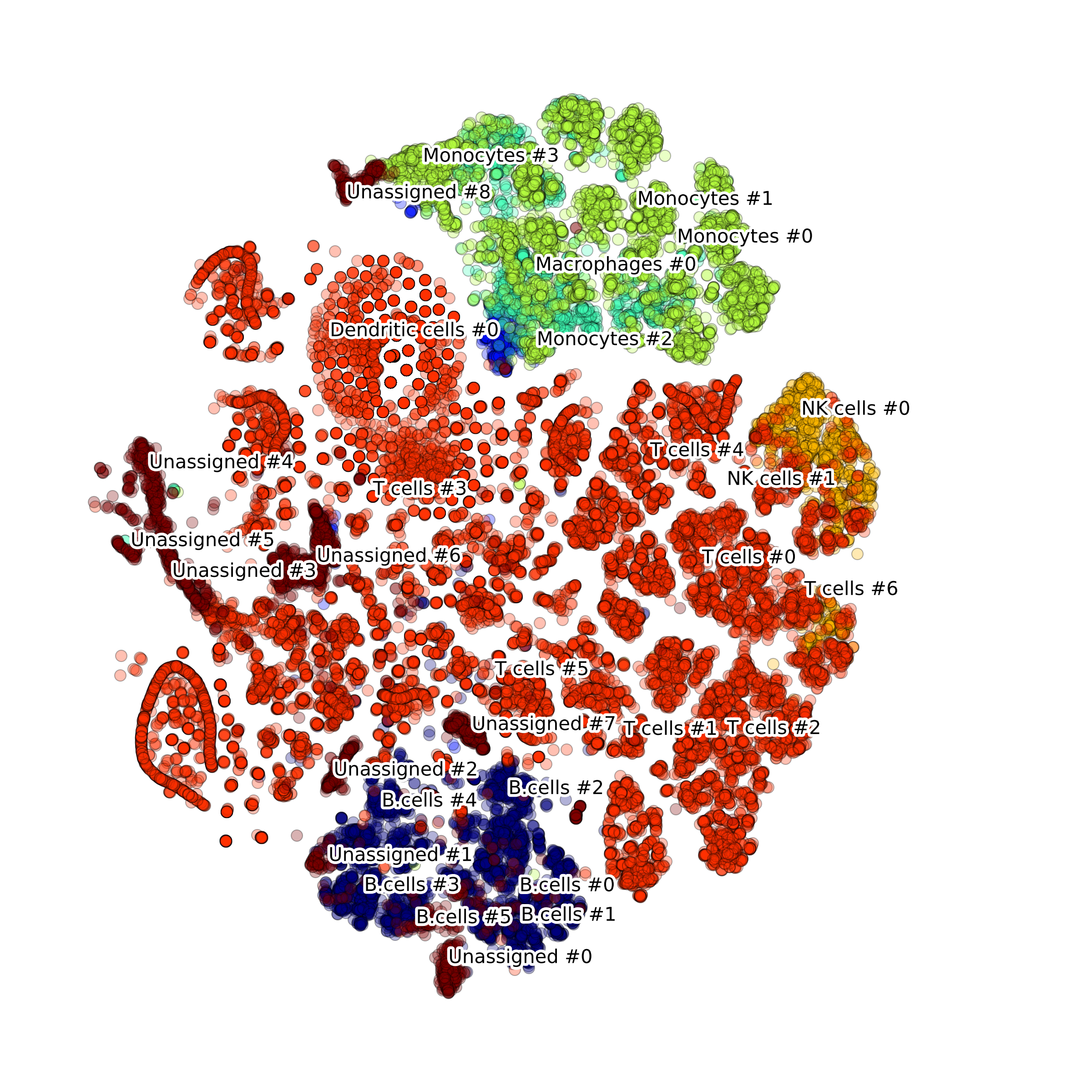
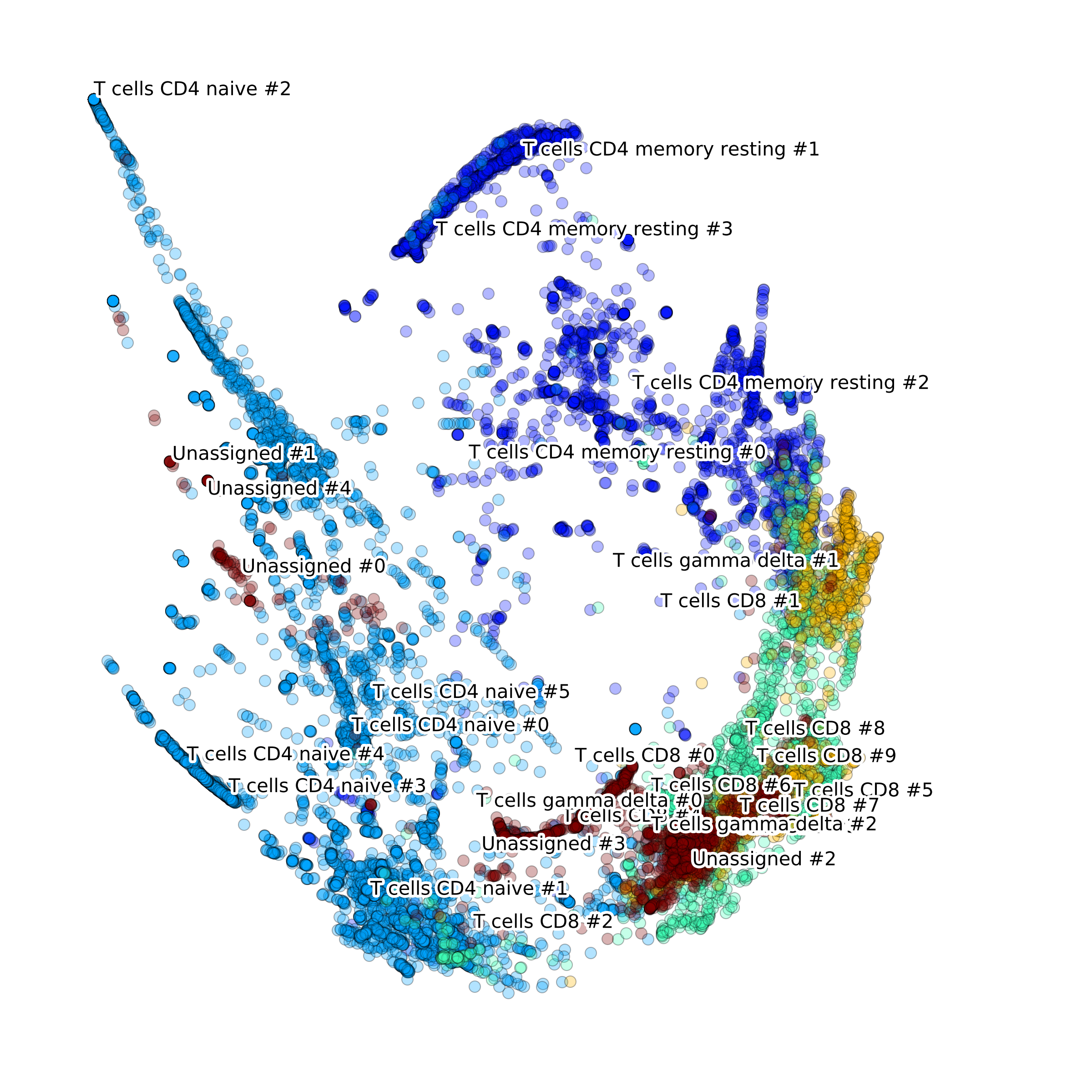
This way the t-SNE layout with annotated clusters (left) of T cell sub-types and the corresponding voting matrix (right)
are generated by the function process():

We can reuse the DCSsub to analyze cell type 'B cell'. Just modify the following attributes:
DCSsub.subclusteringName = 'B cell'
DCSsub.saveDir = os.path.join(os.path.dirname(__file__), 'output', DCS.dataName, 'subclustering B cell', '')
DCSsub.geneListFileName = os.path.join(os.path.dirname(__file__), 'docs', 'examples', 'CIBERSORT_B_SUB.xlsx')

DCSsub.process(df_expr[DCS.getCells(celltype='B cell')])
To execute the complete script demo.py run:
python demo.py
*Note that the HCA BM1 data contains 48000 sequenced cells, requiring approximately 60Gb of RAM (we recommend to use High Performance Computers).
If you want to run our example on a regular PC or a laptop, you can use a randomly chosen number of cells when using HCAtools:
PrepareDataOnePatient(os.path.join('data', 'ica_bone_marrow_h5.h5'), 'BM1', os.path.join('data', ''),
                               useAllData=False, cellsLimitToUse=5000)
Output
All the output files are saved in output directory inside the directory where the demo.py script is.
If you specify any other directory, the results will be generetaed in it.
If you do not provide any directory the results will appear in the root where the script was executed.
Release history Release notifications | RSS feed


Download files
Download the file for your platform. If you're not sure which to choose, learn more about installing packages.
Source Distribution
Built Distribution
Filter files by name, interpreter, ABI, and platform.
If you're not sure about the file name format, learn more about wheel file names.
Copy a direct link to the current filters
File details
Details for the file DigitalCellSorter-1.2.3.tar.gz.
File metadata
- Download URL: DigitalCellSorter-1.2.3.tar.gz
- Upload date:
- Size: 6.1 MB
- Tags: Source
- Uploaded using Trusted Publishing? No
- Uploaded via: twine/2.0.0 pkginfo/1.4.2 requests/2.22.0 setuptools/41.2.0 requests-toolbelt/0.9.1 tqdm/4.28.1 CPython/3.7.1
File hashes
| Algorithm | Hash digest | |
|---|---|---|
| SHA256 |
f76acd9d3ba65cfe1bbc10a2d97fc50303d1c47ecde954e6f9a2b14272d837d2
|
|
| MD5 |
e2f3cdc34d5b577fec650c9430b1dcbf
|
|
| BLAKE2b-256 |
f9f8af4720622e53251f65ae6faaf51c787e81d4c700e5340c75688f895cd22c
|
File details
Details for the file DigitalCellSorter-1.2.3-py3-none-any.whl.
File metadata
- Download URL: DigitalCellSorter-1.2.3-py3-none-any.whl
- Upload date:
- Size: 6.2 MB
- Tags: Python 3
- Uploaded using Trusted Publishing? No
- Uploaded via: twine/2.0.0 pkginfo/1.4.2 requests/2.22.0 setuptools/41.2.0 requests-toolbelt/0.9.1 tqdm/4.28.1 CPython/3.7.1
File hashes
| Algorithm | Hash digest | |
|---|---|---|
| SHA256 |
652fe04601c053860c6c136a89886342dc1ae460fd202253601ce6743e5a6d39
|
|
| MD5 |
bf378bd5afe1165f0602349b9dd11793
|
|
| BLAKE2b-256 |
64393662634a071f41f45e7b16e7f451a6f7bac8d14d3541e12ae340b893e43c
|


