A python toolset for mining multi-dimensional features of the translatome with ribosome profiling data

Project description
RiboMiner
Introduction
The RiboMiner is a python toolset for mining multi-dimensional features of the translatome with ribosome profiling data. This package has four function parts:
- Quality Control (QC): Quality control for ribosome profiling data, containing periodicity checking, reads distribution among different reading frames,length distribution of ribosome footprints and DNA contaminations.
- Metagene Analysis (MA): Metagene analysis among different samples to find possible ribosome stalling events.
- Feature Analysis (FA): Feature analysis among different gene sets identified in MA step to explain the possible ribosome stalling.
- Enrichment Analysis (EA): Enrichment analysis to find possible co-translation events.
Notes:
-
All transcripts used on this package are the longest trancript of all protein coding genes.
-
Codes to reproduce the results presented in the paper are presented in Implementation file or published in CodeOcean for repeatability analysis.
-
Pipelines of Ribominer are also available as a Gene Container Service (GCS) on the Huawei Cloud. Refer to:
-
RiboMiner: Including all functions in RiboMiner. Suitable for most users.
-
RiboMiner-MA: Used for metagene analysis in this study.
-
RiboMiner-FA: Used for feature analysis in this study.
-
RiboMiner-EA: Used for enrichment analysis in this study.
-
Dependencies
- matplotlib>=2.1.0
- numpy>=1.16.4
- pandas>=0.24.2
- pysam>=0.15.2
- scipy>=1.1.0
- seaborn>=0.8.1
- biopython>=1.70
- scipy>=1.1.0
- RiboCode>=1.2.10
- HTSeq
Installation
RiboMiner can be installed like any other Python packages. Here are some popular ways:
- Install via pypi:
pip install RiboMiner
- Install with conda
conda install -c sherking ribominer or
conda install -c bioconda ribominer
- Install from source:
git clone https://github.com/xryanglab/RiboMiner.git
cd RiboMiner
python setup.py install
Usage
Data preparation (DP)
The analysis based on this package need some transcript sequences and annotation file. Before starting the analysis, we need to prepare those files ahead of time. However, the basic annotation file such genome FASTA file, GTF file for annotation which may be used for mapping need to be downloaded by user themselves from Ensemble. Notes: the GTF annotation file should contain 'transcript_type' or 'transcript_biotype' information in the last field.
- Prepare sequences and annotaiton files on transcriptome level.
prepare_transcripts -g <Homo_sapiens.GRCh38.88.gtf> -f <Homo_sapiens.GRCh38.dna.primary_assembly.fa> -o <RiboCode_annot>
The prepare_transcripts is a function of RiboCode, which is used for generated annoation files on transcriptome level. Details please see the manuals of RiboCode. This would generate a directory named RiboCode_annot, containing some annotation file, for example:
transcripts_cds.txt: coordinate file containing transcripts of all protein coding genes.
transcripts_sequence.fa: transcript sequences containing all protein coding transcripts.
- Prepare the longest transcript annotaion files.
OutputTranscriptInfo -c <transcripts_cds.txt> -g <gtfFile.gtf> -f <transcripts_sequence.fa> -o <longest.transcripts.info.txt> -O <all.transcripts.info.txt>
This step would generated two files, one is the longest.transcripts.info.txt, containing annotation infomation of the longest transcripts of all protein coding genes. And the all.transcripts.info.txt containing annotation infomation of all transcripts. The transcripts_sequence.fa was generated by prepare_trascripts, A function of RiboCode.
- Prepare the sequence file for the longest transcripts
GetProteinCodingSequence -i <transcripts_sequence.fa> -c <longest.transcripts.info.txt> -o <output_prefix> --mode whole --table 1 {-l -r -S}
This step would generate three files. One is the amino acid sequences of the longest transcripts. One is the transcript sequences of the longest transcripts. And the last one is the cds sequences of the longest transcripts. transcripts_sequence.fa and longest.transcripts.info.txt are generated above. --table controls which genetic code we should use, default is the standard. If you want to get sequences of a specific gene set, please reset -S parameter. Notes: -S represents transcripts belong to the longest.transcripts.info.txt.
Sometines, UTR sequences are needed. In this case, GetUTRSequences maybe helpful:
GetUTRSequences -i <input_transcript_sequences.fa> -o <output_prefix> -c <transcripts_cds.txt>
where input_transcript_sequences.fa are any transcript sequences you are interested in from transcripts_sequence.fa generated by RiboCode and transcripts_cds.txt are coordinate file generated by RiboCode.
Quality Control (QC)
Quality Control has some basic functions, containing periodicity checking, reads distribution among reading frames,length distribution of ribosome footprints and DNA contamination. Notes: all BAM files used as following should be sorted and indexed.
- Periodicity checking.
Ribosome profiling data with a good quality tend to have a good 3-nt periodicity.
metaplots -a <RiboCode_annot> -r <transcript.bam> -o <output_prefix>
This is a function of RiboCode, and it will generated a pdf file with periodicity of ribosome footprint with different length. In this step, users should record the read length and off-set of reads with a good periodicity, and construct a attributes.txt file in this format (Each columns are separated by TAB):
bamFiles    readLengths Offsets bamLegends
./SRR5008134.bam    27,28,29,30 11,12,13,14 si-Ctrl-1
./SRR5008135.bam    27,28,29,30 11,12,13,14 si-Ctrl-2
./SRR5008136.bam    27,28,29    11,12,13    si-eIF5A-1
./SRR5008137.bam    27,28,29    11,12,13    si-eIF5A-2
The first column is the position and name of your bam files, the second column is the lengths of reads with good periodicity separated by comma, the third column is the off-set separated by comma and the last column is the names of bam file. Also, you could also use the Periodicity in this package to do the same thing but without statistics like this:
Periodicity -i <transcript.bam> -a <RiboCode_annot> -o <output_prefix> -c <longest.transcripts.info.txt> -L 25 -R 35 {-S select_trans.txt --id-type transcript-id}
This step would generated a pdf file containing periodicity of reads with different length from 25 to 35. The transcript.bam is a bam file mapped to transcriptome. longest.transcripts.info.txt is the annotation file generated by OutputTranscriptInfo. This function is transplant from RiboCode but without P-site identification. If the users want to look at the periodicity of a specific gene sets, -S and --id-type could be helpful, the latter is used for control of id type of input transcript sequence. Notes: transcripts in select_trans.txt are a subset of genes from the longest.transcripts.info.txt. And the first column of select_trans.txt must be sequence id corresponding with --id-type and it must has a column name like:
trans_id
ENST00000244230
ENST00000552951
ENST00000428040
ENST00000389682
ENST00000271628
- Reads distribution among different reading frames.
If the ribosome profiling data has a good 3-nt periodicity, the reads of ribosome footprint would be enriched on a specific reading frame. This step is used for statistics of reads covered on different reading frames.
RiboDensityOfDiffFrames -f <attributes.txt> -c <longest.transcripts.info.txt> -o <output_prefix> {-S select_trans.txt --id-type transcript-id --plot yes}
where attributes.txt is constructed by users based on the results of periodicity. And longest.transcripts.info.txt is generated by OutputTranscriptInfo on the step of Data preparation. This step would generated two files for each sample, one is the reads distribution plot with pdf format and the other is the read numbers of different reading frames for each gene.
- Length distribution.
The length distribution of normal ribosome profiling data is around 28nt~30nt, any abnormal length distribution maybe represent problems from library construction or sequencing steps. So this is also an important criterian for data with a good quality.
LengthDistribution -i <sequence_sample.fastq> -o <output_prefix> -f fastq
or
LengthDistribution -i <sequence_sample.bam> -o <output_prefix> -f bam
where sequence_sample.fastq is the fastq file after adapter trimmed and filtered with sequence quality and sequence_sample.bam is the mapping file. This step would generate two files. One is the plot of length distribution with pdf format and the other is the length of each sequencing read.
If users want to display length distribution of reads from differnet regions (CDS, 5'UTR, 3'UTR) or calculate reads length for specific transcripts, ReadsLengthOfSpecificRegions would be helpful.
usage:
ReadsLengthOfSpecificRegions -i bamFile  -c longest.transcripts.info.txt -o output_prefix --type CDS/5UTR/3UTR { -S transcript_list --id-type transcript_id}
- DNA contamination.
Sometimes the length distribution of ribosome footprint is biased away from 28nt-30nt, which is the normal length distribution of ribosome profiling data. Therefore, this step aims to statistic numbers of the reads mapped to RNA, DNA, Intron region,and re-check the length distriution of reads mapped to transcriptome.
StatisticReadsOnDNAsContam -i <genome.bam> -g <gtfFile.gtf> -o <output_prefix>
where genome.bam is bam file mapped to genome, gtfFile.gtf is the genome annotation file such as Homo_sapiens.GRCh38.88.gtf. This step would generated four files, one is the reads distribution of mapped reads <output_prefix_reads_distribution.txt>, like this:
unique mapped reads of exon: 16161306
unique mapped reads of intergenic region: 36937
unique mapped reads of intron: 345
unique mapped ambiguous reads of RNA: 119989
The other three are pdf files, which are length distribution plot of reads mapped to RNA, DNA, and Intron. Notes: this step would consume a lot of time, aroumd 10~20 minutes.
- Read counting
Usage:
ModifyHTseq -i bamFile -g gtfFile -o countsFile -t exon -m union -q 10 --minLen 25 --maxLen 35 --exclude-first 45 --exclude-last 15 --id-type gene_id
Notes: This script only used for strand specific library.
Metagene Analysis (MA)
There are lots of abnormal translation events such as ribosome stalling or ribosome queueing, which would regulate the elongation rate of ribosome moving along transcripts and finally influence the output of protein synthesis. Therefore it is very important to find out the possible ribosome stalling events along transcripts. Metagene analysis is one of ways to do such things.
- Metagene analysis along the whole transcript region.
MetageneAnalysisForTheWholeRegions -f <attributes.txt> -c <longest.transcripts.info.txt> -o <output_prefix> -b 15,90,60 -l 100 -n 10 -m 1 -e 5 --plot yes
MetageneAnalysisForTheWholeRegions is used for metagene analysis along the whole transcript, containing the 5'UTR, CDS, and 3'UTR. The output is a metagene plot with pdf format as well as a density file used for metagene plot. "-b" represents the relative length of 5'UTR,CDS,and 3'UTR, which is separated by comma; "-l" controls the minimum length of transcripts in codon level, 150 codon in default; "-n" controls the minimum read density along transcripts in RPKM filtering mode; "-e" controls numbers of codon that need to be excluded when normalizing the read density with the mean density of a given transcript. "-m" controls the minimum read density of a given transcript after excluding the first "-e" codons; "--plot" controls whether to plot the results.
This step would generate two files, one is the output_prefix_metagenePlot_forTheWholeRegions.pdf and the other is the output_prefix_scaled_density_dataframe.txt used for plot, in which each column is a sample and each row is the position along the transcript with length scaled. Users could use PlotMetageneAnalysisForTheWholeRegions to plot the read density along the transcript based on output_prefix_scaled_density_dataframe.txt file.
PlotMetageneAnalysisForTheWholeRegions -i <output_prefix_scaled_density_dataframe.txt> -o <output_prefix> -g <group1,group2> -r <group1-rep1,group1-rep2__group2-rep1,group2-rep2> -b 15,90,60 --mode all {--ymin,--ymax}
where -g is the group names of samples or conditions which are separated by comma. It is recommmended that the first one is the control group and the next one is treat group. -r is the replicate names corresponding to the -g as well as bamLegends in attributes.txt file. Groups are separated by "__" and the replicates of one groups are separated by comma. -b must be the sample as -b in MetageneAnalysisForTheWholeRegions. --mode controls to output density plot of all samples or just mean density of different replicates.
- Metagene analysis on CDS regions.
There are three ways of input for this function. The first one is that you can input an attributes.txt file which contains all samples including their location, sample name, read length and offset with a -f parameter. The second one is that you could input all samples with -i, -r, -s, -t parameters, all the information are the same as what are included in attributes.txt file. The last one is that you could input the samples one by one with -i, -r, -s, -t parameters and use MergeSampleDensitys to merge all the output files.
## the first way
MetageneAnalysis -f <attributes.txt> -c <longest.transcripts.info.txt> -o <output_prefix> -U codon -M RPKM -u 0 -d 500 -l 100 -n 10 -m 1 -e 5 --norm yes -y 100 --CI 0.95 --type CDS

## the second way
MetageneAnalysis -i ctrl1.bam,ctrl2.bam,treat1.bam,treat2.bam -r 28,29,30_28,29,30_28,29,30_28,29,30 -s 12,12,12_12,12,12_12,12,12_12,12,12 -t ctrl1,ctrl2,treat1,treat2 -c <longest.transcripts.info.txt> -o <output_prefix> -U codon -M RPKM -u 0 -d 500 -l 100 -n 10 -m 1 -e 5 --norm yes -y 100 --CI 0.95 --type CDS

## the third way
MetageneAnalysis -i ctrl1.bam -r 28,29,30 -s 12,12,12 -t ctrl1 -c <longest.transcripts.info.txt> -o <output_prefix> -U codon -M RPKM -u 0 -d 500 -l 100 -n 10 -m 1 -e 5 --norm yes -y 100 --CI 0.95 --type CDS
MetageneAnalysis -i ctrl2.bam -r 28,29,30 -s 12,12,12 -t ctrl2 -c <longest.transcripts.info.txt> -o <output_prefix> -U codon -M RPKM -u 0 -d 500 -l 100 -n 10 -m 1 -e 5 --norm yes -y 100 --CI 0.95 --type CDS
MetageneAnalysis -i treat1.bam -r 28,29,30 -s 12,12,12 -t treat1 -c <longest.transcripts.info.txt> -o <output_prefix> -U codon -M RPKM -u 0 -d 500 -l 100 -n 10 -m 1 -e 5 --norm yes -y 100 --CI 0.95 --type CDS
MetageneAnalysis -i treat2.bam -r 28,29,30 -s 12,12,12 -t treat2 -c <longest.transcripts.info.txt> -o <output_prefix> -U codon -M RPKM -u 0 -d 500 -l 100 -n 10 -m 1 -e 5 --norm yes -y 100 --CI 0.95 --type CDS

## merge all the output files generated by the third way
MergeSampleDensity ctrl1_dataframe.txt,ctrl2_dataframe.txt,treat1_dataframe.txt,treat2_dataframe.txt <output_prefix>
MetageneAnalysis is used for metagene analysis on CDS regions or UTR regions. "--type" controls CDS or UTR, default CDS; "--CI" controls confidence intervals of density at each position; "--norm" controls whether to normalize the read density at each position; "-y" controls how many codons to output for each transcript; "-U" and "-M" controls unit of density calculation and filering mode, respectively; "-u" and "-d" controls the range of CDS region relative to start codon or stop codon. Notes: if "--type" set to be "UTR", the "-U" must be "nt".
This step would generate four kind of files. One is output_prefix_metagenePlot.pdf, a metagene plot of different samples. One is output_prefix_transcript_id.txt, containing all transcripts passed all filtering criteria. One is the output_prefix_dataframe.txt which could be used for generating output_prefix_metagenePlot.pdf and the last one is output_prefix_sampleName_codon_density.txt which is the results of -y, containing ribosome density at each codon or nt for each transcript. Also, we offer a script PlotMetageneAnalysis to plot the metagene plot like this:
PlotMetageneAnalysis -i <output_prefix_dataframe.txt> -o <output_prefix> -g <group1,group2> -r <group1-rep1,group1-rep2__group2-rep1,group2-rep2> -u 0 -d 500 -U codon {--format --ymin --ymax --slide-window --axvline --start --window --step --CI}
where -u ,-d and -U must be corresponding to MetageneAnalysis. And the --slide-window, --start and --window controls whether to smooth the line with a slide-window average method.
- Metagene analysis on UTR regions.
MetageneAnalysis -f <attributes.txt> -c <longest.transcripts.info.txt> -o <output_prefix> -U nt -M RPKM -u 100 -d 100 -l 100 -n 10 -m 1 -e 5 --norm yes -y 50 --CI 0.95 --type UTR
The output of this step is the same as what you did on Metagene analysis on CDS regions
- Polarity calculation.
Polarity values is usually used for judging the ribosome density enriched on 5' end of ORFs or 3' end of ORFs. Values colse to -1, indicating ribosomes enriched more on 3' ORFs and values close to 1, indicating ribosomes enriched more on 5' ORFs.
PolarityCalculation -f <attributes.txt> -c <longest.transcripts.info.txt> -o <output_prefix> -n 64
"-n" controls the minimum read counts of a transcript. And this step would generated a distribution plot of polarity values and could indicate whether ribosomes are enriched or not.
This step would generate two files. One is the distribution plot of polarity values and the other is the file used for generating the plot. And you could also use a extra script PlotPolarity to generate such polarity plot like this:
PlotPolarity -i <output_prefix_polarity_dataframe.txt> -o output_prefix -g <group1,group2> -r <group1-rep1,group1-rep2__group2-rep1,group2-rep2> {-y 5}
This would generate two plot files. One is the distribution plot of polarity for all samples. And the other is the distribution plot of mean polarity among different replicates.
Feature Analysis (FA)
The feature analysis involves some factors which may influence the translation elongation rate, containing tRNA adaptation index (tAI), codon adaptation index (CAI), hydrophobicity of amino acid in new piptide chain, charges of amino acids, poly-Proline motifs, et al.
- Pick out transcripts enriched ribosomes on specific region.
If we found a global ribosome stalling event on a specific region , for example, 25-75 codons. We should pick those transcripts stalled ribosomes out. The RiboDensityForSpecificRegion could be helpful.
RiboDensityForSpecificRegion -f <attributes.txt> -c <longest.transcripts.info.txt> -o <output_prefix> -U codon -M RPKM -L 25 -R 75
This would generate a file containing the mean ribosome density on the specific region (codon 25-75) of all the longest transcripts based on which users could pick those transcripts enriched ribosomes out. And later on, users should use the new gene lists to do the metagene analysis again with a -S parameter and check is there any difference between different gene lists. In this case, only those transcripts enriched ribosomes on the specific region are ready for downstream analysis.
- Ribosome density at each kind of AA or codon.
This step would calculate ribosome density at each kind of codon or amino acid (AA) based on which users could compare density among different codons or AAs and check if the ribosome could have kind of preference along the whole transcript.
RiboDensityAtEachKindAAOrCodon -f <attributes.txt> -c <longest.transcripts.info.txt> -o <output_prefix> -M [counts|RPKM] -S <select_trans.txt> -l 100 -n 10 --table 1 -F <longest_cds_sequence.fa>
Where -S is the transcripts you are interested in. -F is the cds sequences of the longest transcripts generated by GetProteinCodingSequence . Notes: the first column of the select_trans.txt must be the transcripts and with a column name.
The output of this step is a file containing ribosome density at each kind of codon or amino acid like this:
AA      codon   ctrl-1       ctrl-2       treat-1      treat-2
K       AAA     0.026594288206047208    0.029364263341463245    0.015578462857160988    0.014649362490996175
N       AAC     0.023361565164523757    0.025593616862523674    0.025286390202746506    0.025597799715113747
We can also calculate the ribosome density of each kind of AA or codon at a specific region, for example codon 25-75 by add -u and -d parameters.
RiboDensityAtEachKindAAOrCodon -f <attributes.txt> -c <longest.transcripts.info.txt> -o <output_prefix> -M [counts|RPKM] -S <select_trans.txt> -l 100 -n 10 --table 1 -F <longest_cds_sequence.fa> -u 25 -d 75
This would generate two files. One is the ribosome density at the specific region (coodn 25-75)----output_prefix_specific_range_codon_density.txt, the other is the ribosome density out of this region (codon 75-stop codon)----output_prefix_rest_range_codon_density.txt.
- Ribosome density on amino acids with positive or negative charge
Once you got the ribosome density at each kind of codon or AA, use PlotRiboDensityAtEachKindAAOrCodon to plot the density and differences between control groups and treat groups.
PlotRiboDensityAtEachKindAAOrCodon -i <output_prefix_all_codon_density.txt> -o <output_prefix> -g <group1,group2> -r <group1-rep1,group1-rep2__group2-rep1,group2-rep2> --level AA
This step would generate a pdf file containing ribosome density at each kind of AA or codon as for each sample. And there is also a density difference plot among control and treat groups at the last page of the file.
- Pausing score of each triplete amino acid.
Pausing score of each triplete amino acid is the sum of ribosome density covered on this tri-AA motif. And this kind of pausing score could help us find out those tri-AA motifs which could enrich more ribosome.
PausingScore -f <attributes.txt> -c <longest.transcripts.info.txt> -o <output_prefix> -M [counts|RPKM] -S <select_trans.txt> -l 100 -n 10 --table 1 -F <longest_cds_sequence.fa>
The input and parameters are almost the same as RiboDensityAtEachKindAAOrCodon. And it could also offer -L and -R to calculate pausing score of tri-AA motifs at the specific region just like the -u and -d of RiboDensityAtEachKindAAOrCodon did.
This step would generate a pausing score file as for each sample. In order to pick those tri-AA motifs enriched more ribosomes out, we offer ProcessPausingScore to do such job and output an position weight matrix for E,P,A sites of a tri-AA motif which later on could be used for motif logo plot using Seq2Logo.
ProcessPausingScore -i <group1-rep1_pausing_score.txt,group1-rep2_pausing_score.txt,group2-rep1_pausing_score.txt,group2-rep2_pausing_score.txt> -o <output_prefix> -g <group1,group2> -r <group1-rep1,group1-rep2__group2-rep1,group2-rep2> --mode [raw|ratio] --ratio_filter 2 --pausing_score_filter 10
Where -i is the pausing score file we need to input, and all pausing score file should be separated by comma. --ratio_filter 2 means the FC(treat/ctrl)>=2 and --pausing_score_filter 10 means pausing score on treat group must be larger than 10. --mode raw means input is the raw pausing score generated by PausingScore; --mode ratio means input is the processed file with this format:
motif	si-Ctrl	si-eIF5A	ratio
PPP	9.583728008472916	32.40390126709601	3.3811374069097035
DDD	7.864248366516	18.973658903418116	2.4126474672650478
SPP	5.095062641097612	14.244816613232201	2.7958079451921103
LPP	6.269550858040044	13.567581067294325	2.1640435454631204
DDP	3.533105599301455	13.297017644747527	3.763549452746766
APP	3.8178063397299846	11.921477030003814	3.1225986781841226
And the last position weight matrix looks like this:
        A	D	L	P	S
0	0.14909086080045236	0.4526622484437558	0.10332391327033515	0.16143499003013836	0.13348798745531829
1	0.0	0.45266224844375585	0.0	0.5473377515562442	0.0
2	0.0	0.1367730692993923	0.0	0.8632269307006076	0.0
Where the 0,1,2 represent the E,P,A site of a tri-AA motif. Using Seq2Logo for logo plot:
## this tool needs a python2.7 environment
PATH=/tools/python2:$PATH
Seq2Logo.py -f <pwm.txt> -u probability -I 5 -o <output_preifx> --format PDF
-
Ribosome density around the triplete amino acid (tri-AA) motifs.
Now that we have find out tri-AA motifs enriched more ribosomes, we want to know the ribosome density around those tri-AA motifs and check whether there are any differences between the control and treat groups on those motifs.
- As for a specific tri-AA motif, such as poly-proline (PPP)
RiboDensityAroundTripleteAAMotifs -f <attributes.txt> -c <longest.transcripts.info.txt> -o PPP -M [RPKM|counts] -S <select_trans.txt> -l 100 -n 10 --table 1 -F <longest_cds_sequence.fa> --type2 PPP --type1 PPIn this case, it would generate a file named PPP_motifDensity_dataframe.txt which could be used for plot of ribosome density around PPP or NPP motifs using PlotRiboDensityAroundTriAAMotifs like this:
PlotRiboDensityAroundTriAAMotifs -i PPP_motifDensity_dataframe.txt -o PPP -g <group1,group2> -r <group1-rep1,group1-rep2__group2-rep1,group2-rep2> --mode mean- As for a tri-AA motifs list which contains part of information like this:
motifs
PPP
DDD
SPP
LPP
Using following command to do such job:
RiboDensityAroundTripleteAAMotifs -f <attributes.txt> -c <longest.transcripts.info.txt> -o <output_prefix> -M [RPKM|counts] -S <select_trans.txt> -l 100 -n 10 --table 1 -F <longest_cds_sequence.fa> --motifList1 tri_AA_motifs1.txt --motifList2 tri_AA_motifs2.txtThis would generate a file containing ribosome density of all tri-AA motifs in tri_AA_motifs1.txt and tri_AA_motifs2.txt. Later on use the same command to plot.
-
RPFdist calculation.
RPFdist defines as the ratio of ribosome density on 5'UTR and density on CDS region. And usually it is negatively correlated with translation efficiency (TE).
RPFdist -f <attributes.txt> -c <longest.transcripts.info.txt> -o <output_prefix> -M [RPKM|counts] -S <select_trans.txt> -l 100 -n 10 -m 1 -e 5
- GC contents for sequences with a fasta format.
There are two kinds of mode for GC contents calculation. normal mode: calculate GC contents for a given sequence (GC/total). frames mode: calculate GC contents of each reading frame for a given sequence.
GCContent -i <input_sequences.fa> -o <output_prefix> --mode [normal|frames]
After this step, use PlotGCContent to get statistic plot of GC contents for the given sequences.
## normal mode
PlotGCContent -i <output_prefix_GC_content.txt> -o <output_prefix> --mode normal
## frames mode
PlotGCContent -i <output_prefix_GC_content_frames.txt> -o <output_prefix> --mode frames
- Local tRNA adaptation index and global tRNA adaptation index
This step would generate two file. One is the file containing the local tAI values at each positon along transcripts and the other contains the global tAI values.
tAI -i <cds_sequence_1.fa,cds_sequence_2.fa...> -o <output_prefix> -t <geneList1,geneList2...> -u 0 -d 500 --table 1 -N <tRNA_gene_copy_numbers.txt>
where the tRNA_gene_copy_numbers.txt is the file downloaded from GtRNAdb with this format:
Chr	tRNA	Begin	End	Isotype	Anticodon	Upstream	Downstream
chr6	95	58141949	58141877	Ala	AGC	tttctccctc	gtttcttgtc
chr6	25	26751918	26751990	Ala	AGC	agtgtagtgt	gcttctttta
chr1	87	150017452	150017382	Ala	AGC	aagaattaaa	caaaggtttt
chr6	94	58142661	58142589	Ala	AGC	agtgtagtgt	gcttctttta
chr6	160	26773843	26773771	Ala	AGC	atgcggtgtg	gcttctttta
chr6	23	26728256	26728328	Ala	AGC	atgcggtgtg	gcttctttta
where the Anticodon column is a must. After this step, we could use tAIPlot for local tAI plot with:
tAIPlot -i <output_prefix_tAI_dataframe.txt> -o <output_prefix> -u 0 -d 500 --mode all --start 5 --window 7 --step 1
- Local codon adaptation index and global codon adaptation index
As for CAI calculation, we need a reference sequences to calculate frequency of each codon or relative synonymous codon usage (RSCU) values from very highly expressed genes of the organism.
cAI -i <cds_sequence_1.fa,cds_sequence_2.fa...> -o <output_prefix> -t <geneList1,geneList2...> -u 0 -d 500 [--RSCU <RSUCs.txt> | --reference <references.fa> | --weight <weight.txt>]
Where -i are the input sequences with fasta format separated by comma. -t are the sequence lengends corresponding to the input sequences. --reference is a reference sequences highly expressed in a specific organism. --RSCU and --weight are weight files containing weight of each codon. And this step would generate two files. One is the local cAI,and the other is the global codon adaptation index. Part codes were from CAI package developed by Lee, B. D.
After this step, we could use cAIPlot to plot the local cAI values with a metagene method.
cAIPlot -i <output_prefix_local_cAI_dataframe.txt> -o <output_prefix> -u 0 -d 500 --mode all --start 5 --window 7 --step 1
Notice that the cds sequences for a specific gene list could be generated by GetProteinCodingSequence like:
GetProteinCodingSequence -i <transcrits_sequence.fa> -c <longest.trans.info.txt> -S <select_trans.txt> -o <output_prefix> --mode whole --table 1 --id-type transcript-id
- Hydrophobicity calculation and Charge amino acids
hydropathyCharge could be used for hydrophobicity calculation as well as charges of amino acid by set --index to a related index file.
## hydrophobicity calculation
hydropathyCharge  -i <cds_sequence_1.fa,cds_sequence_2.fa...> -o <output_prefix> -t <geneList1,geneList2...> --index <hydrophobicity_index.txt> -u 0 -d 500 --table 1
##
hydropathyCharge  -i <cds_sequence_1.fa,cds_sequence_2.fa...> -o <output_prefix> -t <geneList1,geneList2...> --index <charge_index.txt> -u 0 -d 500 --table 1
the both index file looks like:
## hydrophobicity index download from AAindex
AA	amio_acids	hydropathy
A	Ala 	1.8
R	Arg 	-4.5
N	Asn 	-3.5
D	Asp 	-3.5
C	Cys 	2.5
...
## charge index
AA	amio_acids	charge
A	Ala 	0
R	Arg 	1
N	Asn 	0
D	Asp 	-1
C	Cys 	0
Q	Gln 	0
E	Glu 	-1
G	Gly 	0
H	His 	1
...
among which the hydrophobicity index are downloaded from AAindex. Later on, use PlotHydropathyCharge for plot:
## hydrophobicity
PlotHydropathyCharge -i <output_prefix_hydropathy_dataframe.txt> -o <output_prefix> -u 0 -d 500 --mode all --ylab "Average Hydrophobicity"
## charge
PlotHydropathyCharge -i <output_prefix_charge_values_dataframe.txt> -o <output_prefix> -u 0 -d 500 --mode all --ylab "Average Charges"
Enrichment Analysis (EA)
The enrichment analysis is used for identifying potential co-translation events just like Ayala Shiber, et al did. Therefore, there are two input files for this step. One is the total translatome file and the other is the IP translatome file. The enrichment analysis contains four steps:
- Step 1: Calculate ribosome density at each position for each transcript.
RiboDensityAtEachPosition -c <longest.transcripts.info.txt> -f <attributes.txt> -o <output_prefix> -U [codon|nt]
where attributes.txt and longest.transcripts.info.txt are files we have talked above. This step would generate two files for each sample. One is the ribosome density file which would be used for following analysis. The Other is the coverage file, containing coverage of each transcript on CDS region.
- Step 2: Calculate mean ribosome density for different replicates.
enrichmentMeanDensity -i rep1-density.txt,rep2-density.txt,rep3-density.txt -o <output_prefix>
-i represents ribosome density files of different replicates generated by RiboDensityAtEachPosition, which should be separated by comma. This would generate a mean density file for each sample like output_prefix_mean_density.txt, used for enrichment analysis. If there is no replicates, just pass this step.
- Step 3: Enrichment analysis.
## all transcripts
EnrichmentAnalysis --ctrl <total-translatome.txt> --treat <IP-translatome.txt> -c <longest.transcripts.info.txt> -o <output_prefix> -U codon -M RPKM -l 150 -n 10 -m 1 -e 30 --CI 0.95 -u 0 -d 500

## specific transcripts
EnrichmentAnalysis --ctrl <total-translatome.txt> --treat <IP-translatome.txt> -c <longest.transcripts.info.txt> -o <output_prefix> -U codon -M RPKM -l 150 -n 10 -m 1 -e 30 --CI 0.95 -u 0 -d 500 -S <select_trans.txt>
Where --ctrl represents ribosome density for total translatome sample and --treat represents ribosome density for IP translatome sample, both of which could be generated by RiboDensityAtEachPosition in Step 1 or Step 2. This step would generate three files. One is the output_prefix_enrichment_dataframe.txt used for plot. One is the output_prefix_enrichment_transcript_id.txt, representing transcripts that passed the filtering criteria. And the last one is output_prefix_ratio.txt, representing enrichment ratio at each position for those transcripts passed filtering criteria.
- Step 4: Plot the enrichment ratio.
PlotEnrichmentRatio -i <enrichment_dataframe.txt> -o <output_prefix> -u 0 -d 500 --unit codon --mode all {--slide-window y --axvline 1 --axhline 60 --label legend_label}
where enrichment_dataframe.txt was generated by EnrichmentAnalysis in Step 3. --slide-window y controls whether to smooth the curves with the slide-average method or not.
- Notes: if you want to see the enrichment ratio for a single transcript, the EnrichmentAnalysisForSingleTrans would be helpful.
EnrichmentAnalysisForSingleTrans -i <output_prefix_codon_ratio.txt> -s <transcript_name> -o <output_prefix> -c <longest.trans.info.txt> --id-type transcript_id --slide-window y --axhline 1
where the output_prefix_codon_ratio.txt was generated by EnrichmentAnalysis in Step 3; transcript_name is the single transcript you are interested in, and either transcript id or gene name or gene id for that transcript was required.This step would generate a plot file with pdf format. And if you set -S rather than -s with a transcript list file input, the output file would be a pdf file containing plots for each transcript.
Others
RiboMiner could offer other useful functions that would help users analyze ribosome profiling data, such as statistics of read coverage, visualization of read density for a single transcript or some transcript sets.
- Read Coverage
CoverageOfEachTrans -f <attributes.txt> -c <longest.transcripts.info.txt> -o <output_prefix> --mode coverage {-S select_trans.txt --id-type transcript-id}
This would generate two ouput files for each sample presented in attributes.txt. One is output_prefix_sample_raw_depth.txt and the other is output_prefix_sample_RPM_depth.txt. -S parameter is an optional setting, which means you can choose to output coverage of your interested transcripts. If -S is not available, it will output read coverage of all transcripts by default. Using another script PlotTransCoverage to visualize read coverage of you interested transcript:
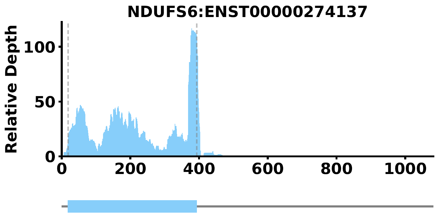
PlotTransCoverage -i <output_prefix_sample_RPM_depth.txt> -o NDUFS6 -c <longest.transcripts.info.txt> -t NDUFS6 --mode coverage --id-type gene_name --color lightskyblue --type single-gene
where --type single-gene means output a pdf plot only containing read coverage for a single gene or transcript, such as NDUFS6. if --type gene-list -S select_genes.txt are set, it will ouput a pdf with multiple plots for read coverage of transcripts. The plot is like this:
- Read Density
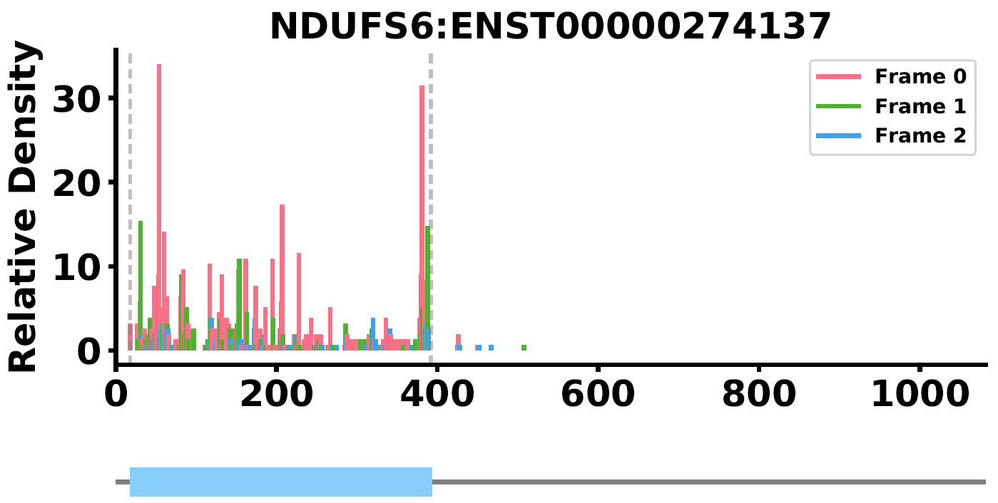
CoverageOfEachTrans -f <attributes.txt> -c <longest.transcripts.info.txt> -o <output_prefix> --mode density {-S select_trans.txt --id-type transcript-id}
where --mode density means output of read density of transcripts rather than coverage. It will also generate two files: output_prefix_sample_raw_density.txt and output_prefix_sample_RPM_density.txt. Using PlotTransCoverage to visualize read density of you interested transcript:
PlotTransCoverage -i <output_prefix_sample_RPM_density.txt> -o NDUFS6 -c <longest.transcripts.info.txt> -t NDUFS6 --mode density --id-type gene_name --color lightskyblue --type single-gene
where different colors in the density plot means different open reading frames of NDUFS6 transcript, which may show a 3-nt periodicity.
Implementation
Details for Implementation, please refer to Implementation.
Release history Release notifications | RSS feed


Download files
Download the file for your platform. If you're not sure which to choose, learn more about installing packages.
Source Distribution
Built Distribution
Filter files by name, interpreter, ABI, and platform.
If you're not sure about the file name format, learn more about wheel file names.
Copy a direct link to the current filters
File details
Details for the file RiboMiner-0.2.3.2.1.tar.gz.
File metadata
- Download URL: RiboMiner-0.2.3.2.1.tar.gz
- Upload date:
- Size: 3.9 MB
- Tags: Source
- Uploaded using Trusted Publishing? No
- Uploaded via: twine/3.4.2 importlib_metadata/4.8.1 pkginfo/1.6.1 requests/2.24.0 requests-toolbelt/0.9.1 tqdm/4.50.2 CPython/3.8.5
File hashes
| Algorithm | Hash digest | |
|---|---|---|
| SHA256 |
18325c19c972b4dc979f8cb9e7d6ec50cb2fce289cdbb1a7553e7264a35b5414
|
|
| MD5 |
a79b42814f7ce30d2660d5dd563d59d5
|
|
| BLAKE2b-256 |
95ca3de3a9f49c46ef1173169c8f7f19e38303e8fa662046285072a4a31ea80a
|
File details
Details for the file RiboMiner-0.2.3.2.1-py3-none-any.whl.
File metadata
- Download URL: RiboMiner-0.2.3.2.1-py3-none-any.whl
- Upload date:
- Size: 143.8 kB
- Tags: Python 3
- Uploaded using Trusted Publishing? No
- Uploaded via: twine/3.4.2 importlib_metadata/4.8.1 pkginfo/1.6.1 requests/2.24.0 requests-toolbelt/0.9.1 tqdm/4.50.2 CPython/3.8.5
File hashes
| Algorithm | Hash digest | |
|---|---|---|
| SHA256 |
906df2be7688dd6b8d5f71f69bd53b7441b150ec03724be1c47880d89be5f1a5
|
|
| MD5 |
06578da6199196f71d9d890986c48987
|
|
| BLAKE2b-256 |
97ec5ec2fc48590ec20b421094841789a56a2e3551063689933b1e1302af0050
|


