Synthetic biochemical reaction networks with definable degree distributions.

Project description
SBbadger
SBbadger is a Python library for the generation of synthetic, directed, reaction networks that conform to user-defined degree distributions.
Documentation
https://SBbadger.readthedocs.io
Quick Start
Installation
Supported versions of Python are 3.7, 3.8, and 3.9. Python dependencies include numpy, scipy, antimony, matplotlib, and pydot. An additional dependency for pydot is either a system installation of Graphviz or pydot installation via conda.
SBbadger can be installed using pip:
$ pip install SBbadger
Simple Example
In the simplest possible case SBbadger can generate a single, 10 species, random network using the following commands in the python interpreter:
>>> from SBbadger import generate
>>> generate.models()
Note to Windows users. Currently the above won't work on windows in a script file. To use the package on windows in a script file you must use:
from SBbadger import generate

if __name__ == "__main__":
   generate.models()
This will be fixed in a future version.
In this case, SBbadger will randomly select reactions from 4 possible reaction types and randomly select the reactants and products for those reactions from the 10 species. The possible reaction types are:
| Reaction Type | Default Probabilities | Examples |
|---|---|---|
| UNI-UNI | 0.35 | A -> B |
| BI-UNI | 0.3 | A + B -> C |
| UNI-BI | 0.3 | A -> B + C |
| BI-BI | 0.05 | A + B -> C + D |
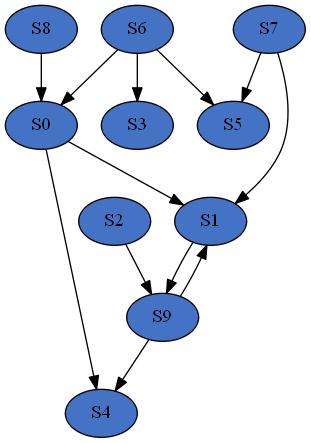
The default reaction probabilities are adjustable. Also note that the same species can be chosen more than once in a reaction, for example A + A -> B is a valid reaction. Reactions will continue to be added to the network until all 10 species have included. Below is the depiction of a sample network and an Antimony string describing the associated model:
var S0, S1, S9
ext S2, S3, S4, S5, S6, S7, S8

J0: S8 -> S0; kc0*S8
J1: S6 -> S5 + S0; kc1*S6
J2: S2 + S1 -> S9; kc2*S2*S1
J3: S7 -> S1 + S5; kc3*S7
J4: S9 + S0 -> S1 + S4; kc4*S9*S0
J5: S6 -> S3; kc5*S6

kc0 = 0.10285116762815472
kc1 = 65.21087405102236
kc2 = 34.220083386257116
kc3 = 11.526991028714853
kc4 = 0.15553486234310213
kc5 = 4.977089372937806

S2 = 4.759074353180305
S3 = 1.666194306431944
S4 = 7.110932299198714
S5 = 6.803821600602985
S6 = 9.329699040726386
S7 = 7.7760175494627735
S8 = 9.74931761300573

S0 = 3.431293190721635
S1 = 5.5106455586766545
S9 = 7.631625970757748
var and ext denote floating and boundary species respectively. The default
rate law is mass action with all parameters randomly selected from a log-uniform
distribution with a range from 0.001 to 100. Initial conditions are randomly selected
from a uniform distribution with a range from 0 to 10. By default, the reactions are
irreversible.
Expanded Example
Now suppose we want to create many models, and with more defined properties. The following python script will do just that.
from SBbadger import generate
from scipy.stats import zipf

def in_dist(k):
    return k ** (-2)

def out_dist(k):
    return zipf.pmf(k, 3)

if __name__ == "__main__":

    generate.models(
		group_name="extended_example",
		n_models=10,
		n_species=100,
		in_dist=in_dist,
		out_dist=out_dist,
		min_freq=1.0,
		n_cpus=4
		)
Two distribution functions are defined, in_dist and out_dist, for the in-edge and out-edge distributions respectively where k is the degree. Both are power law functions. SBbadger will discretize, truncate, and renormalize these functions.
Note that in_dist is defined explicitly but out_dist is a wrapper around the Scipy function zipf. A short description of the other parameters follows:
group_name: prepended to all files and the name of the directory where those files will be deposited.n_models: The number of models to be produced.n_species: The number of nodes/species per model.min_freq: The minimum expected frequency of nodes in every bin. This parameter, along with the number of species, is used to determine where to truncate the distribution.n_cpus: The number of cores to run in parallel. Note thatif __name__ == "__main__":is necessary to use multiprocessing on Windows.
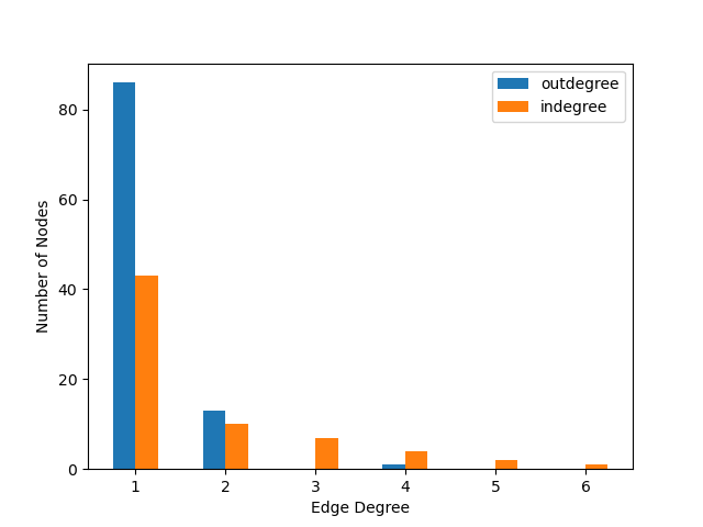
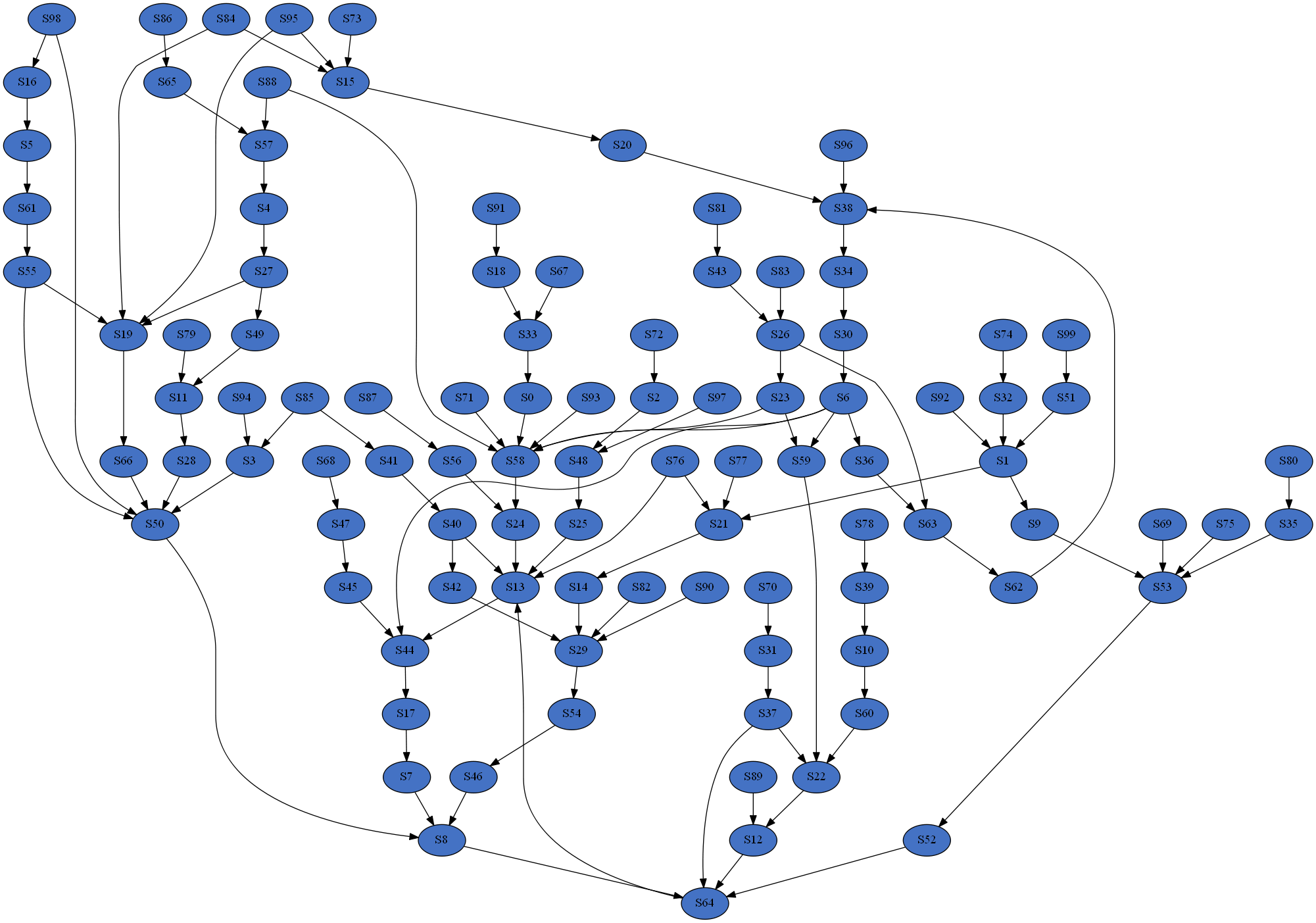
In the above example 10 models will be produced, each with 100 species; the in-edge and out-edge distributions will both follow a power law but with different exponents; the distributions will be truncated such that every degree bin will have a minimum expected node count of 1; and the models will be split into 4 groups to be processed in parallel. Below are examples of the resulting distributions and a network.
Release history Release notifications | RSS feed


Download files
Download the file for your platform. If you're not sure which to choose, learn more about installing packages.
Source Distribution
File details
Details for the file SBbadger-1.4.5.tar.gz.
File metadata
- Download URL: SBbadger-1.4.5.tar.gz
- Upload date:
- Size: 54.1 kB
- Tags: Source
- Uploaded using Trusted Publishing? No
- Uploaded via: twine/4.0.2 CPython/3.7.16
File hashes
| Algorithm | Hash digest | |
|---|---|---|
| SHA256 |
022dc3b3335e4d58e72daa3ca0b6528037b8f7132ea502db449c71ea78a630ea
|
|
| MD5 |
c7b7649914f9d2ff5ce7c436aece8b6a
|
|
| BLAKE2b-256 |
5970d09e83b63e24a40e3e1b485037022d113e4bad5d316006ac9607868870e5
|


