Interactive python tool designed to label radio emission features of interest in a temporal-spectral map

Project description
SPACE Labelling Tool V2.0.0


The SPectrogram Analysis and Cataloguing Environment (SPACE) tool is an interactive python tool designed to label radio emission features of interest in a temporal-spectral map (called “dynamic spectrum”). The Software uses Matplotlib’s Polygon Selector widget to allow a user to select and edit an undefined number of vertices on top of the dynamic spectrum before closing the shape (polygon). Multiple polygons may be drawn on any spectrum, and the feature name along with the coordinates for each polygon vertex are saved into a “.json” file as per the “Time-Frequency Catalogue” (TFCat) format along with other data such as the feature id, observer name, and data units. This paper describes the first official stable release (version 2.0) of the tool.
SPACE is part of the MASER (Measuring Analyzing & Simulating Emissions in Radio frequencies) project.
Getting Started
Clone this repository, and then install it in 'editable' mode as:
git clone https://github.com/CorentinLouis/SPACE_labelling_tool.git
pip install -e SPACE_labelling_tool
Installing in editable mode will allow the scripts to read any new or modified versions of the configuration files.
SPACE Labelling Tool is also directly available from PyPi: https://pypi.org/project/space-labelling-tool/
pip install SPACE-labelling-tool
Usage
spacelabel [-h] [-s SPACECRAFT] FILE DATE DATE
Positional arguments:
FILE: The name of the.hdf5or.cdffile to analyse. It must be in the format outlined in the data_dictionary; three (or more) columns!DATE: The window of days to plot, in ISO YYYY-MM-DD format, e.g. '2003-12-01 2003-12-31' for December 2003. The data will be scrolled through in blocks of this window's width.
Optional arguments:
-h,--help: Shows help documentation.-s SPACECRAFT: The name of the spacecraft. Auto-detected from the input file columns, but required if multiple spacecraft describe the same input file.-f FREQUENCY: How many log-space frequency bins to rebin the data to. Overrides any default for the spacecraft.-t TIME_MINIMUM: How small the minimum time bin should be, in seconds. This must be an even multiple of the current time bins, e.g. a file with 1s time bins could have a minimum time bin of 15s.-fig_size FIGURE_SIZE FIGURE_SIZE: x and y dimension of the matplotlib figure (by default: 15 9)-frac_dyn_range FRAC_DYN_RANGE FRAC_DYN_RANGE: The minimum and maximum fraction of the flux to be display in the dynamic range (by default: 0.05 0.95)-cmap CMAP: The name of the color map that will be used for the intensity plot (by default: viridis)-cfeatures CFEATURES: The name of the colour for the saved features of interest polygons (by default: tomato)-thickness_features TFEATURES: The thickness value for the saved features of interest polygons (by default: 2)-size_features_name SFEATURESNAME: The font size for the name of the saved features of interest polygons (by default: 14)-g [FREQUENCY_GUIDE [FREQUENCY_GUIDE ...]]: Draws horizontal line(s) on the visualisation at these specified frequencies to aid in interpretation of the plot.Values must be in the same units as the data.Lines can be toggled using check boxes.--not_verbose: If not_verbose is called, the debug log will not be printed. By default: verbose mode
The code will attempt to identify which spacecraft the data file format corresponds to, and read the file intelligently. If it can't fit one of them, it will prompt the user to create a new spacecraft configuration file. In the case of a file matching multiple spacecraft formats, the user is prompted to select one.
GUI
Once the file has loaded, it launches a GUI for selecting the measurements within the file to display, and then to navigate the data selected. The plot will display the time range selected, plus 1/4 of the previous window.
There are the following interactive components:
-
Measurements: Each pane displays a measurement, with name, scale and units on the right. Features can be drawn by clicking to add coordinates, and completed by clicking on the first coordinate added again. The vertices of the polygon can be modified before completed the polygon:
- Hold ctrl and click and drag a vertex to reposition it before the polygon has been completed.
- Hold the shift key and click and drag anywhere in the axes to move all vertices.
- Press the esc key to start a new polygon.
Once selected, a feature can be named. Features can be selected on any pane, and will be mirrored on all other panes.
-
Prev/Next buttons: These move through the data by an amount equal to the width of time range selected. This will also overlap 1/4 of the current window as 'padding'.
-
Save button: This will save any features to TFcat JSON format, as
catalogue_{OBSERVER_NAME}.json. -
Check boxes: If the option
-g [FREQUENCY GUIDE [FREQUENCY GUIDE ...]]has been enabled by the users to plot fixed frequency line(s) in the matplotlib window, or if a 1D variable is contained in the input data and configuration files check boxes will appear in the lower right hand corner of the figure to make the white dotted lines appear or disappear.
Once finished, you can save and then close the figure using the normal close button.
Usage Examples
hdf5file Calling the code as:
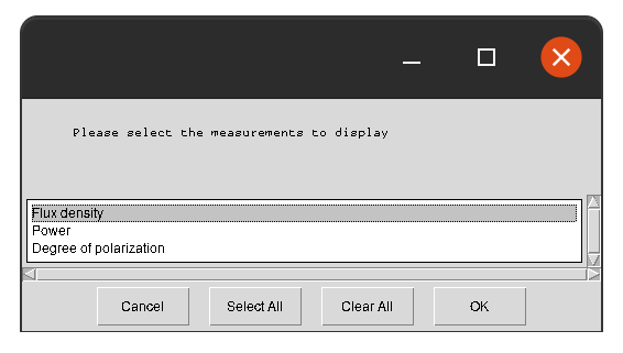
space_label.py cassini_data.hdf5 2006-02-10 2006-02-11 -g 600
Will load the file cassini_data.hdf5, and prompt the user to select which measurements to display:
Once selected, the radio observations will be displayed for the time window 10/2/2006 to 11/2/2006:
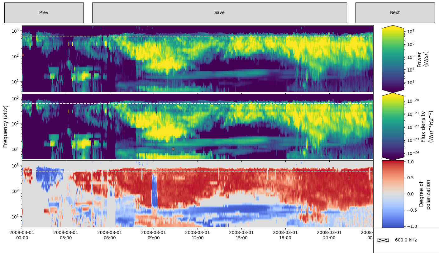
The user can then draw polygon in one panel. The Figure below show Intensity (top panel) and Polarization (bottom panel) data. At the top right of the top panel one can see a polygon that has just been drawn and closed, with the window for naming the feature appearing at the top left of the graphics window. Features can be selected on any pane, and will be mirrored on all other panes once named. Other features have already been labelled, and appear in both intensity and polarisation views, with their names overlaid.

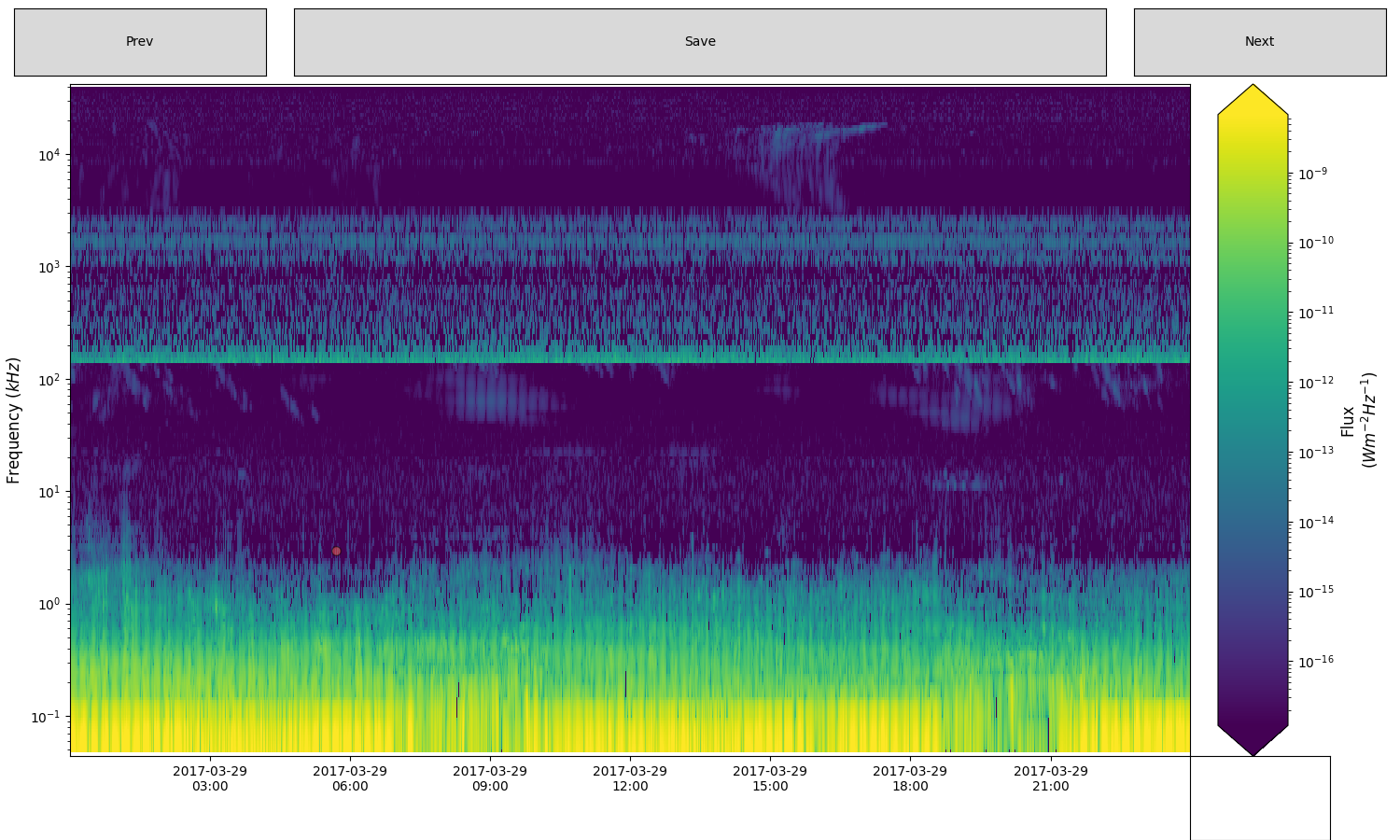
cdffile Calling the code as:
space_label.py juno_data.cdf 2017-03-29 2017-03-30
Will first load the file juno_data.cdf, processed it into hdf5 file (according to the juno.json config file), and then radio observations will be displayed for the time window 29/03/2017 to 30/03/2017:
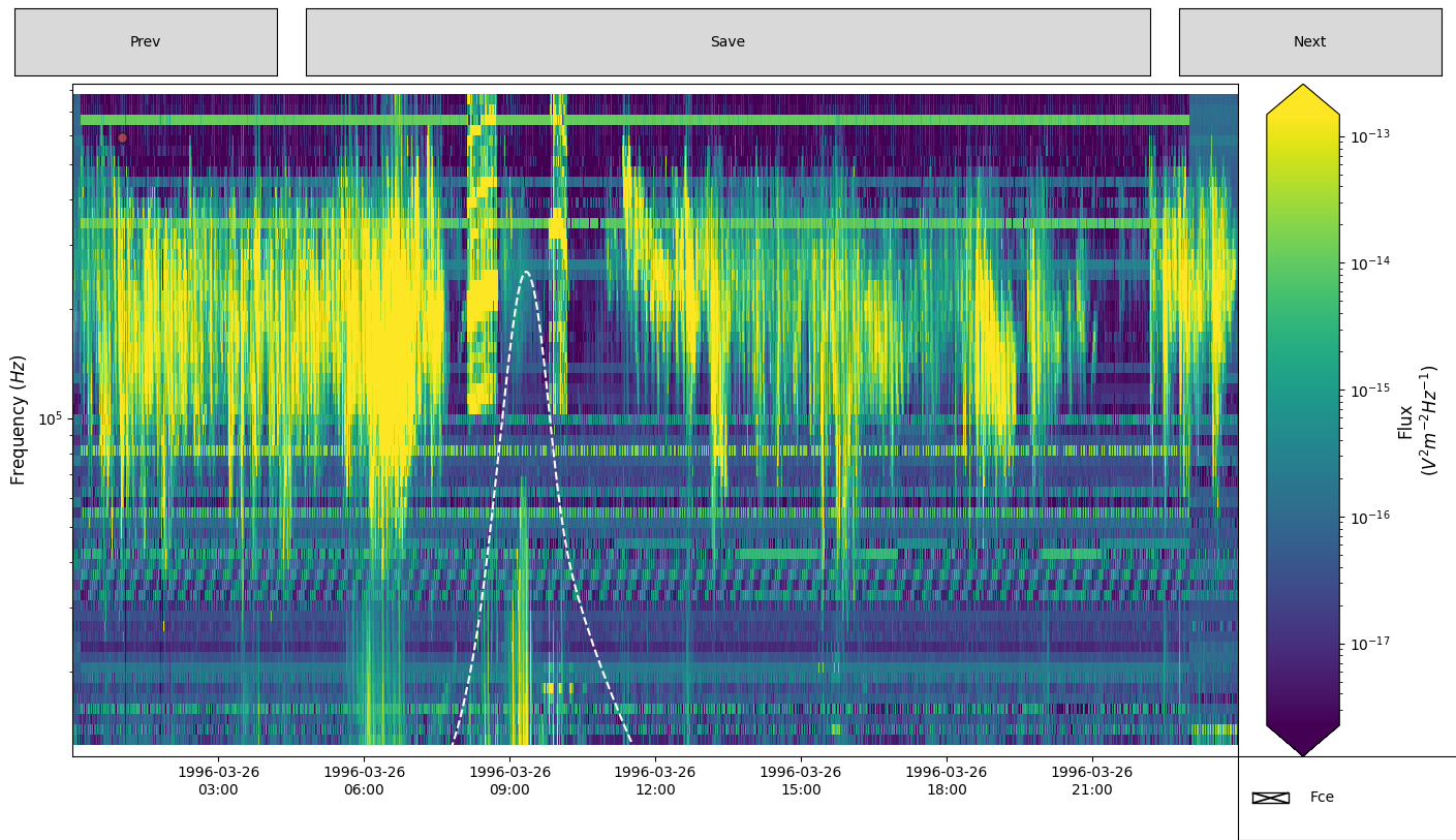
An other example of a cdf file that also contains 1D data (displayed as a white-dashed line):
space_label.py polar_data.cdf 2017-03-29 2017-03-30
Will first load the file polar_data.cdf, processed it into hdf5 file (according to the polar.json config file), and then radio observations will be displayed for the time window 26/03/1996 to 27/03/1996:
Documentation
Readthedocs documentation is accessible here.
Spacecraft configuration files are stored in the config/ directory in JSON format.
For more info on how to create a new one, see spacecraft configurations.
Information on the file formats this program inputs and outputs can be found in the data dictionary.
Limitations & Future Work
- The performance of the MatPlotLib-based front-end is poor for high-resolution plots. Future work would involve re-implementing the front-end in a more modern library like Plotly.
- The code loads all the data provided into memory at launch. This limits its scalability.
Future work would involve re-saving provided data as
parquetor other time-indexable files for partial loads using the Dask and XArray libraries. - Add configurations that load data directly from catalogues.
Terminology
- 'Polarization' has been chosen over 'Polarisation' as it is the Oxford standard for the spelling.
Release history Release notifications | RSS feed

Download files
Download the file for your platform. If you're not sure which to choose, learn more about installing packages.
Source Distribution
Built Distribution
Filter files by name, interpreter, ABI, and platform.
If you're not sure about the file name format, learn more about wheel file names.
Copy a direct link to the current filters
File details
Details for the file SPACE labelling tool-2.0.tar.gz.
File metadata
- Download URL: SPACE labelling tool-2.0.tar.gz
- Upload date:
- Size: 25.8 kB
- Tags: Source
- Uploaded using Trusted Publishing? No
- Uploaded via: twine/4.0.1 CPython/3.8.5
File hashes
| Algorithm | Hash digest | |
|---|---|---|
| SHA256 |
16b24e1ff36fdbe7bae00cfb6f983db555d0b03519e1e002537c25ceeb218cd8
|
|
| MD5 |
2ec56e99ac69d229c816a8244e501e1f
|
|
| BLAKE2b-256 |
3116cee8f3357e02028a13d9cc8aca6e57e889ba6e982b23885112b734ffe985
|
File details
Details for the file SPACE_labelling_tool-2.0-py3-none-any.whl.
File metadata
- Download URL: SPACE_labelling_tool-2.0-py3-none-any.whl
- Upload date:
- Size: 31.1 kB
- Tags: Python 3
- Uploaded using Trusted Publishing? No
- Uploaded via: twine/4.0.1 CPython/3.8.5
File hashes
| Algorithm | Hash digest | |
|---|---|---|
| SHA256 |
ea1afd31c1f36db1c77c230d60a477cfa040f97aaf35d2f4533eef87ad6e1309
|
|
| MD5 |
f6091db5a913e09784c6ee5992202f7f
|
|
| BLAKE2b-256 |
90ae8d1b693f85c0bc72c5aadb636ead897a4bdcf073d7599174bb3a41b22d15
|


