A Python package providing a high-performant C++ implementation of benchmark functions for mathematical optimization algorithms.

Project description


BenchmarkFcns
Benchmarkfcns is an effort to provide a high-performant, public and free implementation of well-known benchmark functions for mathematical optimization algorithms in Python. The Python library is implemented in C++ and utilizes powerful SIMD vector calculations combined with multi-core parallel processing (via OpenMP) to offer extremely fast and efficient evaluation of functions on massive datasets.
For the documentation of the implemented functions and their features, please visit https://benchmarkfcns.info.
Key Features
- High Performance: Optimized C++ core using Eigen and OpenMP.
- Parallel Execution: Automatic multi-core processing for large batches of data.
- SIMD Optimized: Leverages modern CPU instruction sets for fast vector math.
- AI Ready: Standardized Gymnasium (OpenAI Gym) environments for RL training.
- Optimizer Agnostic: Designed for seamless integration with SciPy, PyGMO, and Nevergrad.
- Comprehensive Library: 310+ functions including Classic (100+), CEC suites (2005-2022), Multi-Fidelity (49), and Multi-Objective (50).
- CEC Competition Suites: Built-in support for official CEC 2005, 2014, 2017, 2019, 2020, and 2022 competition functions with embedded shift, rotation, and shuffle data.
- Parallel Composition Engine: Advanced framework for creating hybrid landscapes, now fully parallelized for high-performance batch evaluations.
How to use
Python
Installation
The library is packaged and available on the PyPI index. To install, simply run pip install benchmarkfcns.
Parallel Execution
By default, the library uses all available CPU cores to evaluate large matrices of data points. You can control the number of threads used by setting the OMP_NUM_THREADS environment variable:
# Limit to 4 threads
export OMP_NUM_THREADS=4
python your_script.py
For large-scale tasks (e.g., evaluating 10 million points), this parallel implementation can provide up to 10x-30x speedup compared to single-threaded or pure NumPy implementations.
Usage
After installing, using the library is straightforward and all that is needed is to import the needed functions, construct a matrix of input values and call the function. It should be noted that all the functions in the library only accept matrices as input. The rows of the matrix represent the data points at which the function should be evaluated and the columns represent the dimensions of data points. The code snippet shows how to use the library.
# Import the needed function.
from benchmarkfcns import rastrigin
import numpy as np

# Look at the function's documentation.
print(rastrigin.__doc__)

# The input matrix can be list of lists.
data = [[0, 0, 0]]

# Evaluate the Rastrigin function at (0, 0, 0).
results = rastrigin(data)
print(results)

# The input can also be a Numpy matrix.
data = np.array([[0, 0, 0], [1, 1, 1]])
results = rastrigin(data)
print(results)
Integration with External Optimizers
BenchmarkFcns is designed to be the high-performance fitness engine for established optimization libraries. By leveraging our C++ backend's support for batch evaluations, you can significantly accelerate the optimization process.
Detailed integration scripts can be found in the examples/ directory, covering:
- SciPy: Global optimization with
differential_evolution(including vectorized mode). - Nevergrad: Meta AI's toolbox for derivative-free optimization.
- Optuna: Hyperparameter optimization and Bayesian search.
- Pymoo: Multi-objective optimization (NSGA-II, NSGA-III, etc.).
- CMA-ES: The gold standard for continuous black-box optimization.
Quick Example: SciPy (Vectorized)
from scipy.optimize import differential_evolution
from benchmarkfcns import ackley
import numpy as np

# benchmarkfcns handles the entire population in parallel via OpenMP
result = differential_evolution(ackley, bounds=[(-32, 32)]*10, vectorized=True)
print(f"Global Minimum: {result.fun}")
AI & Reinforcement Learning
The library provides (planned) standardized Gymnasium environments to train RL agents on complex landscapes.
import gymnasium as gym
import benchmarkfcns.environments

# Create an Ackley environment for RL training
env = gym.make("BenchmarkFcns/Ackley-v0", dims=10)
Plotting the functions
This library is implemented to be as compatible as possible with all the mainstream plotting libraries. As a result, you are free to select your favourite plotting library to plot the functions in this library.
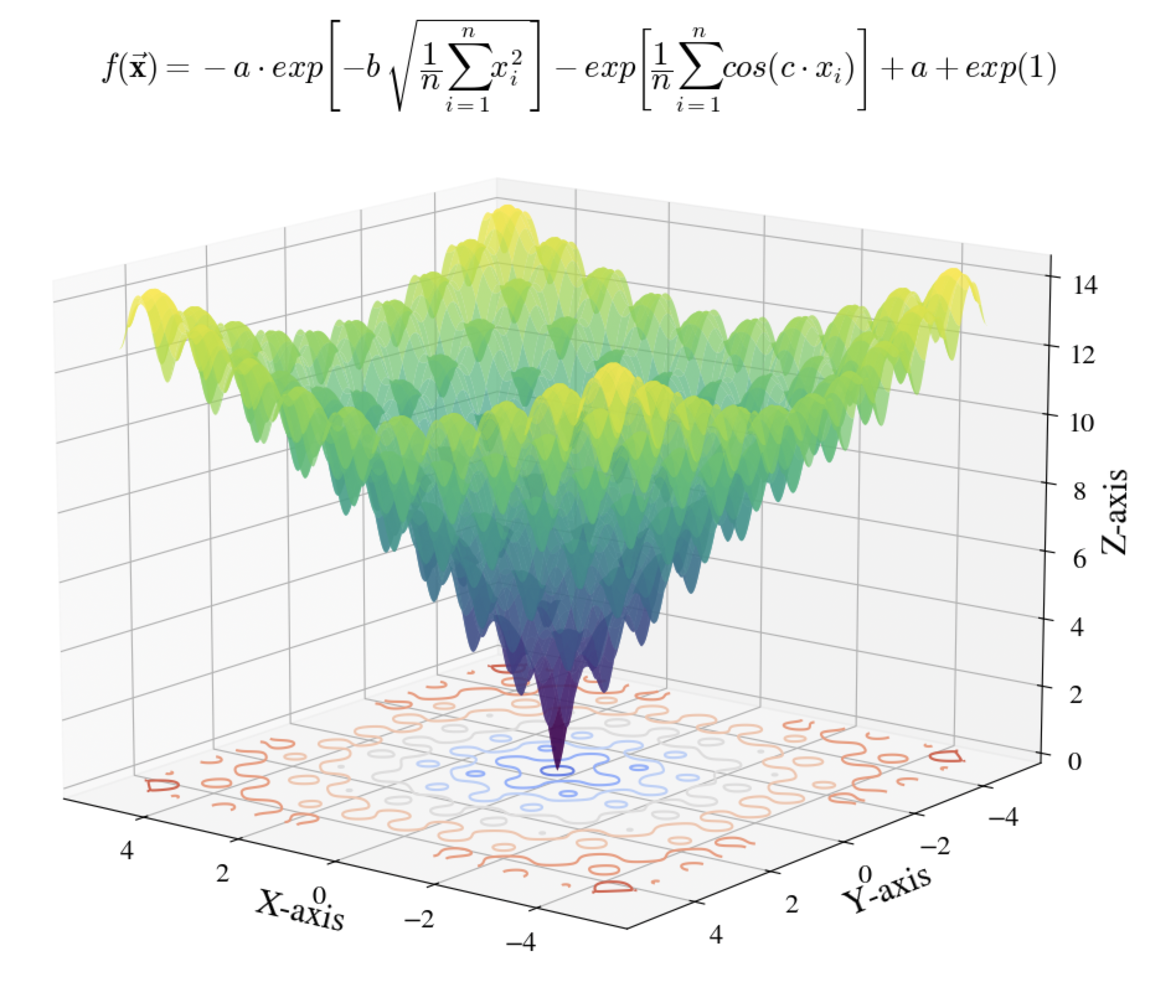
Plotting a mathematical function like rastrigin requires evaluating the function at a rather large set of data points. This is where the vectorized implementation of the functions in this package can shine as it allows performing the evaluations in a single function call, which significantly speeds up the plotting and reduces the computation cost. To facilitate this, the library also contains a helper function, meshgrid, for drawing 3D plots using the vectorized implemetations of the mathematical functions in this library. Given a list of x and y coordinates and a function, this function creates a meshgrid of points, evaluates the function over the meshgrid and returns the corresponding x, y and z points of the meshgrid that can be plotted with any plotting library.
from benchmarkfcns import ackley
from benchmarkfcns.plotting import meshgrid

# Using the matplotlib library for this example
import matplotlib.pyplot as plt
import numpy as np

# Used to make title equation look nicer
import matplotlib
matplotlib.rcParams['mathtext.fontset'] = 'cm'
matplotlib.rcParams['font.family'] = 'STIXGeneral'

# We want to plot the function for x and y in range [-5, 5].
# This corresponds to a grid of 100,000,000 points.
x = np.linspace(-5, 5, 10000)
y = np.linspace(-5, 5, 10000)

# `meshgrid` creates the 3D meshgrid and evaluates `ackley` on it.
# Evaluation of 100,000,000 points took less than 3 seconds.
X, Y, Z = meshgrid(x, y, ackley)

# Create the plot
fig = plt.figure()
ax = fig.add_subplot(111, projection='3d')

# Plot the surface and its contour with a colormap
ax.plot_surface(X, Y, Z, cmap='viridis', alpha=0.7)
ax.contour(X, Y, Z, zdir='z', offset=0, cmap='coolwarm')

# Set labels and title
ax.set_xlabel('X-axis')
ax.set_ylabel('Y-axis')
ax.set_zlabel('Z-axis')
plt.suptitle(r"$f({\bf \vec{x}}) = -a\cdot exp\left[-b\,\sqrt{\dfrac{1}{n}\sum_{i=1}^{n}x_{i}^{2}}\right]-exp\left[\dfrac{1}{n}\sum_{i=1}^{n}cos(c\cdot x_{i})\right]+ a + exp(1)$")

# Set view angle and display
ax.view_init(14, 120)
plt.show()
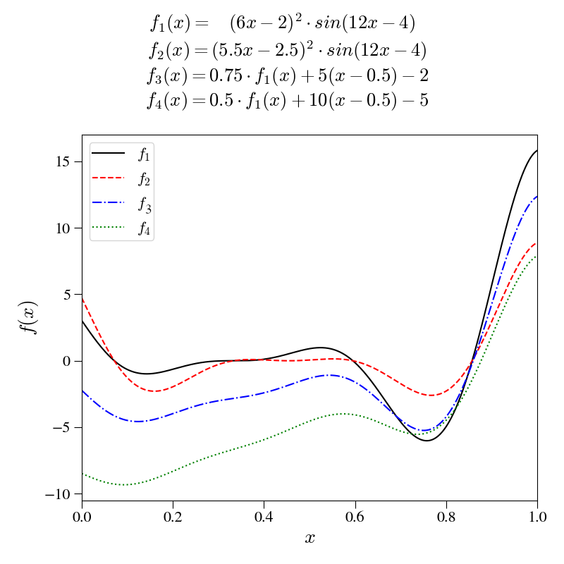
Plotting Multi-fidelity Functions
Addition of multi-fidelity functions such as the forrester function, shown below.
import benchmarkfcns.multifidelity as mfb

# Using the matplotlib library for this example
import matplotlib.pyplot as plt
import numpy as np

# Used to make title equation look nicer
import matplotlib
matplotlib.rcParams['mathtext.fontset'] = 'cm'
matplotlib.rcParams['font.family'] = 'STIXGeneral'

# We want to plot the function for x in range [0, 1].
x = np.linspace(0, 1, 10000)

# Evaluation of points took less than 340 \mu\,s, per function.
f = mfb.forrester(x)

# Create the plot
fig = plt.figure(figsize=(8,8))
ax = fig.add_subplot(111)

# Plot all 4 fidelity levels.
ax.plot(x, f[:, 0], 'k-', label=r"$f_{1}$")
ax.plot(x, f[:, 1], 'r--', label=r"$f_{2}$")
ax.plot(x, f[:, 2], 'b-.', label=r"$f_{3}$")
ax.plot(x, f[:, 3], 'g:', label=r"$f_{4}$")

# Add labels, limits, and legend.
ax.set_xlabel(r"$x$")
ax.set_ylabel(r"$f(x)$")
ax.set_xlim(0,1)
ax.set_ylim(-10.5,17)

plt.suptitle(
    r"$f_{1}(x) =~~~(6x - 2)^{2} \cdot sin(12x - 4)$"
    + f"\n"
    + r"$~~f_{2}(x) = (5.5x - 2.5)^{2} \cdot sin(12x - 4)$"
    + f"\n"
    + r"$~~f_{3}(x) = 0.75 \cdot f_{1}(x) + 5(x - 0.5) - 2$"
    + f"\n"
    + r"$~~f_{4}(x) = 0.5 \cdot f_{1}(x) + 10(x - 0.5) - 5$"
    )

plt.legend()
plt.tight_layout()
plt.show()
Advanced Composition Engine
BenchmarkFcns includes a powerful Composition Engine that allows you to create complex, hybrid benchmark landscapes (similar to those found in the CEC competition suites) by blending multiple base functions.
The engine supports:
- Shifting: Move the local optimum of any component to a specific point.
- Rotation: Apply coordinate rotation matrices to create non-separable challenges.
- Scaling: Stretch or shrink individual component landscapes.
- Exponential Blending: Automatically blends functions based on their distance from their centers using CEC-standard weighting.
Example: Custom Composition
import benchmarkfcns as bf
import numpy as np

# Create a new composition
comp = bf.Composition()

# Add a rotated and shifted Ackley component
n = 10
shift = np.random.uniform(-5, 5, n)
rotation = np.eye(n) # You can provide any orthogonal matrix here
comp.add("ackley", shift=shift, rotation=rotation, sigma=1.0, bias=0.0)

# Add a shifted Rastrigin component with a bias
shift2 = np.random.uniform(-5, 5, n)
comp.add("rastrigin", shift=shift2, sigma=1.0, bias=100.0)

# Evaluate a batch of points
X = np.random.uniform(-5, 5, (100, n))
scores = comp(X)
Example: CEC 2005 Presets
The library provides pre-configured factories for standard competition functions.
import benchmarkfcns as bf

# Create the standard CEC 2005 F15 Hybrid Composition Function
f15 = bf.cec2005_f15(dimensions=10)

X = np.random.uniform(-5, 5, (50, 10))
results = f15(X)
Example: CEC Competition Functions
The library includes full support for multiple CEC Single-Objective suites with official data embedded in the binary.
from benchmarkfcns import cec
import numpy as np

# Evaluate CEC 2017 Function 11 (Hybrid Function 1) for a 10D point
x = np.random.uniform(-100, 100, (1, 10))
score_2017 = cec.evaluate_2017(x, fid=11)

# Evaluate CEC 2022 Function 1 (Zakharov)
score_2022 = cec.evaluate_2022(x, fid=1)
Example: Multi-objective Optimization
The multiobjective submodule provides 50 standard problems including the MaF suite.
from benchmarkfcns import multiobjective
import numpy as np

# Evaluate MaF1 (Inverted DTLZ1) with 3 objectives
x = np.random.uniform(0, 1, (10, 10))
scores = multiobjective.maf1(x, num_objectives=3) # Returns (10, 3) matrix
MATLAB
As a reference, the repository also contains the implementation of the functions in MATLAB. To install and use the MATLAB implementation, it is just required to add the project folders to MATLAB's path. For example, to use the functions in the 'benchmarks/MATLAB' folder, just navigate to this folder with MATLAB's directory explorer or use the command addpath with path to the folder on your PC (e.g. addpath /path/to/benchmarks).
Local development and compilation
The library is built with the pybind11, scikit-build-core and Eigen libraries. To compile the library, you will need to have CMake version 3.15 or above installed and configured. The easiest way to compile and install the package locally is to clone the repository into a directory, e.g. BenchmarkFcns, with submodules initialized using git submodule update --init --recursive, and then run pip install ./BenchmarkFcns. Although optional, it is highly recommended to install the package into a virtual environment.
Contribution
Any suggestions and contributions are welcomed. The best way to contribute to the library is to fork the repository, apply the contributions and create a pull request.
Support
Any bug reports, code contributions, suggestions, feedback and insights are greatly appreciated. If you are using this library in a research publication, please kindly consider citing the repository using the following:
-
For the general reference of the repository:
Mazhar Ansari Ardeh and cmutnik. (2025). Benchmarkfcns. Zenodo. https://doi.org/10.5281/zenodo.14556621 -
For the latest version of the repository (v3.8.0):
Mazhar Ansari Ardeh and cmutnik. (2026). Benchmarkfcns (version v3.8.0). Zenodo. https://doi.org/10.5281/zenodo.18912792
Release history Release notifications | RSS feed


Download files
Download the file for your platform. If you're not sure which to choose, learn more about installing packages.
Source Distribution
File details
Details for the file benchmarkfcns-4.1.0.tar.gz.
File metadata
- Download URL: benchmarkfcns-4.1.0.tar.gz
- Upload date:
- Size: 71.1 MB
- Tags: Source
- Uploaded using Trusted Publishing? Yes
- Uploaded via: twine/6.1.0 CPython/3.13.12
File hashes
| Algorithm | Hash digest | |
|---|---|---|
| SHA256 |
2251a443c71f932c31e832764c691f2fcbdc2714ff727610055f8786eb44c236
|
|
| MD5 |
ce8c34e48c802684a58427bb0991e2a9
|
|
| BLAKE2b-256 |
3d211d0566e9430d33778a834c513526c70d65265b711353568e086b9e24dba2
|
Provenance
The following attestation bundles were made for benchmarkfcns-4.1.0.tar.gz:
Publisher:
build.yaml on mazhar-ansari-ardeh/BenchmarkFcns
-
Statement:
-
Statement type:
https://in-toto.io/Statement/v1 -
Predicate type:
https://docs.pypi.org/attestations/publish/v1 -
Subject name:
benchmarkfcns-4.1.0.tar.gz -
Subject digest:
2251a443c71f932c31e832764c691f2fcbdc2714ff727610055f8786eb44c236 - Sigstore transparency entry: 1569240067
- Sigstore integration time:
-
Permalink:
mazhar-ansari-ardeh/BenchmarkFcns@68ce0b6519cf4277334c481fc1012608d8647163 -
Branch / Tag:
refs/tags/v4.1.0 - Owner: https://github.com/mazhar-ansari-ardeh
-
Access:
public
-
Token Issuer:
https://token.actions.githubusercontent.com -
Runner Environment:
github-hosted -
Publication workflow:
build.yaml@68ce0b6519cf4277334c481fc1012608d8647163 -
Trigger Event:
release
-
Statement type:


