






Machine learning based causal inference/uplift in Python
causeinfer is a Python package for estimating average and conditional average treatment effects using machine learning. The goal is to compile causal inference models both standard and advanced, as well as demonstrate their usage and efficacy - all this with the overarching ambition to help people learn causal inference techniques across business, medical, and socioeconomic fields. See the documentation for a full outline of the package including the available models and datasets.
Contents
- Installation
- Application
- Evaluation Methods
- Data and Examples
- Development environment
- To-Do
- References
Installation
causeinfer is available for installation via uv (recommended) or pip.
For Users
# Using uv (recommended - fast, Rust-based installer):
uv pip install causeinfer

# Or using pip:
pip install causeinfer
For Development Build
git clone https://github.com/andrewtavis/causeinfer.git
cd causeinfer

# With uv (recommended):
uv sync --all-groups  # install all dependencies
source .venv/bin/activate  # activate venv (macOS/Linux)
# .venv\Scripts\activate  # activate venv (Windows)

# Or with pip:
python -m venv .venv  # create virtual environment
source .venv/bin/activate  # activate venv (macOS/Linux)
# .venv\Scripts\activate  # activate venv (Windows)
pip install -e .
import causeinfer
Application
Standard Algorithms
Two Model Approach
Separate models for treatment and control groups are trained and combined to derive average treatment effects (Hansotia, 2002).
from causeinfer.standard_algorithms.two_model import TwoModel
from sklearn.ensemble import RandomForestClassifier, RandomForestRegressor

tm_pred = TwoModel(
    treatment_model=RandomForestRegressor(**kwargs),
    control_model=RandomForestRegressor(**kwargs),
)
tm_pred.fit(X=X_train, y=y_train, w=w_train)

# An array of predictions given a treatment and control model
tm_preds = tm_pred.predict(X=X_test)

tm_proba = TwoModel(
    treatment_model=RandomForestClassifier(**kwargs),
    control_model=RandomForestClassifier(**kwargs),
)
tm_proba.fit(X=X_train, y=y_train, w=w_train)

# An array of predicted treatment class probabilities given models
tm_probas = tm.predict_proba(X=X_test)
Interaction Term Approach
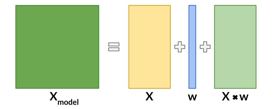
An interaction term between treatment and covariates is added to the data to allow for a basic single model application (Lo, 2002).
from causeinfer.standard_algorithms.interaction_term import InteractionTerm
from sklearn.ensemble import RandomForestClassifier, RandomForestRegressor

it_pred = InteractionTerm(model=RandomForestRegressor(**kwargs))
it_pred.fit(X=X_train, y=y_train, w=w_train)

# An array of predictions given a treatment and control interaction term
it_preds = it_pred.predict(X=X_test)

it_proba = InteractionTerm(model=RandomForestClassifier(**kwargs))
it_proba.fit(X=X_train, y=y_train, w=w_train)

# An array of predicted treatment class probabilities given interaction terms
it_probas = it_proba.predict_proba(X=X_test)
Class Transformation Approaches
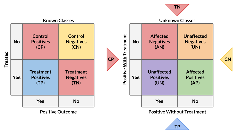
Units are categorized into two or four classes to derive treatment effects from favorable class attributes (Lai, 2006; Kane, et al, 2014; Shaar, et al, 2016).
# Binary Class Transformation
from causeinfer.standard_algorithms.binary_transformation import BinaryTransformation
from sklearn.ensemble import RandomForestClassifier

bt = BinaryTransformation(model=RandomForestClassifier(**kwargs), regularize=True)
bt.fit(X=X_train, y=y_train, w=w_train)

# An array of predicted probabilities (P(Favorable Class), P(Unfavorable Class))
bt_probas = bt.predict_proba(X=X_test)
# Quaternary Class Transformation
from causeinfer.standard_algorithms.quaternary_transformation import (
    QuaternaryTransformation,
)
from sklearn.ensemble import RandomForestClassifier

qt = QuaternaryTransformation(model=RandomForestClassifier(**kwargs), regularize=True)
qt.fit(X=X_train, y=y_train, w=w_train)

# An array of predicted probabilities (P(Favorable Class), P(Unfavorable Class))
qt_probas = qt.predict_proba(X=X_test)
Reflective and Pessimistic Uplift
Weighted versions of the binary class transformation approach that are meant to dampen the original model's inherently noisy results (Shaar, et al, 2016).
# Reflective Uplift Transformation
from causeinfer.standard_algorithms.reflective import ReflectiveUplift
from sklearn.ensemble import RandomForestClassifier

ru = ReflectiveUplift(model=RandomForestClassifier(**kwargs))
ru.fit(X=X_train, y=y_train, w=w_train)

# An array of predicted probabilities (P(Favorable Class), P(Unfavorable Class))
ru_probas = ru.predict_proba(X=X_test)
# Pessimistic Uplift Transformation
from causeinfer.standard_algorithms.pessimistic import PessimisticUplift
from sklearn.ensemble import RandomForestClassifier

pu = PessimisticUplift(model=RandomForestClassifier(**kwargs))
pu.fit(X=X_train, y=y_train, w=w_train)

# An array of predicted probabilities (P(Favorable Class), P(Unfavorable Class))
pu_probas = pu.predict_proba(X=X_test)
Advanced Algorithms
Models to Consider
- Under consideration for inclusion in causeinfer:
- Generalized Random Forest via the R/C++ grf - Athey, Tibshirani, and Wager (2019)
- The X-Learner - Kunzel, et al (2019)
- The R-Learner - Nie and Wager (2017)
- Double Machine Learning - Chernozhukov, et al (2018)
- Information Theory Trees/Forests - Soltys, et al (2015)
Evaluation Methods
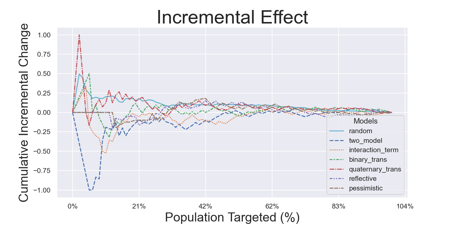
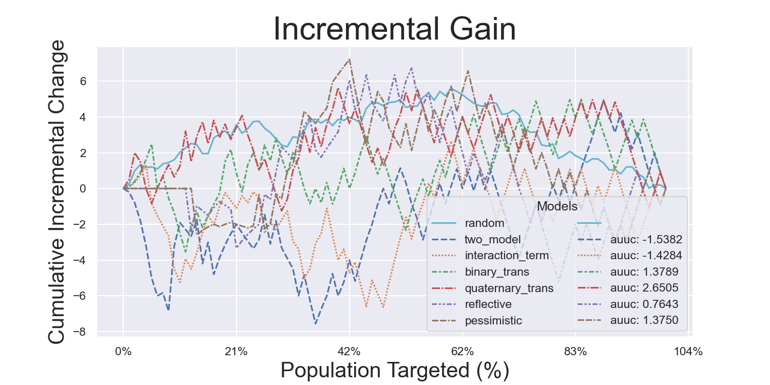
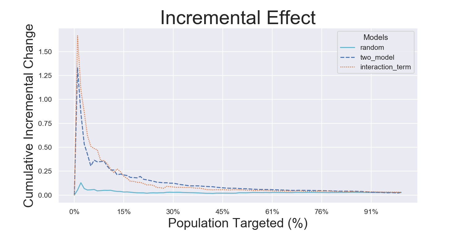
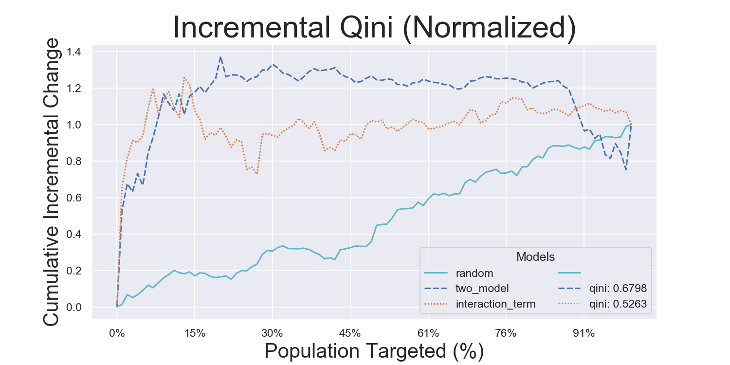
Visualization Metrics and Coefficients
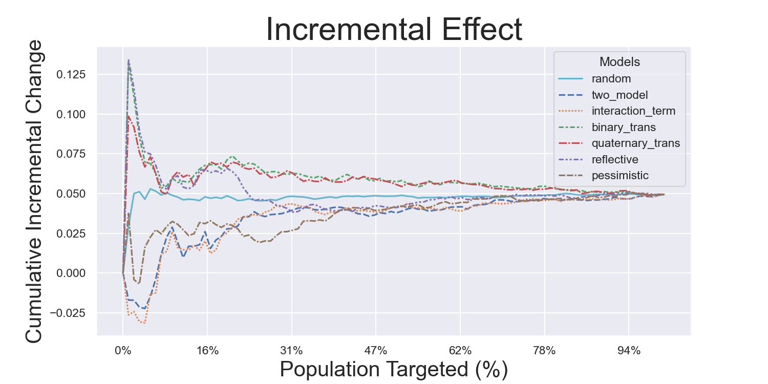
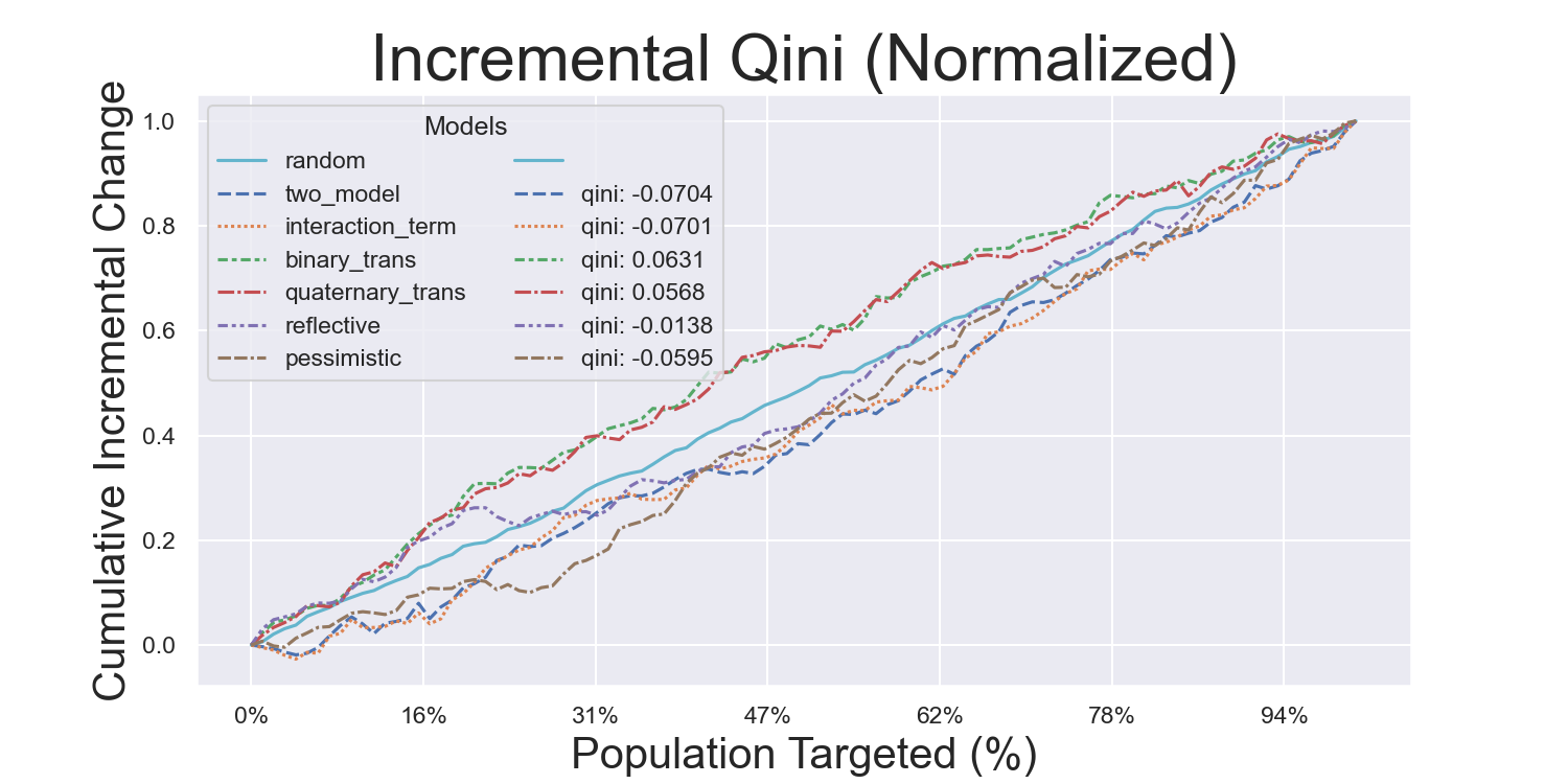
Comparisons across stratified, ordered treatment response groups are used to derive model efficiency.
from causeinfer.evaluation import plot_cum_gain, plot_qini

visual_eval_dict = {
    "y_test": y_test,
    "w_test": w_test,
    "two_model": tm_effects,
    "interaction_term": it_effects,
    "binary_trans": bt_effects,
    "quaternary_trans": qt_effects,
}

df_visual_eval = pd.DataFrame(visual_eval_dict, columns=visual_eval_dict.keys())
model_pred_cols = [
    col for col in visual_eval_dict.keys() if col not in ["y_test", "w_test"]
]
fig, (ax1, ax2) = plt.subplots(ncols=2, sharey=False, figsize=(20, 5))

plot_cum_effect(
    df=df_visual_eval,
    n=100,
    models=models,
    percent_of_pop=True,
    outcome_col="y_test",
    treatment_col="w_test",
    normalize=True,
    random_seed=42,
    axis=ax1,
    legend_metrics=True,
)

plot_qini(  # or plot_cum_gain
    df=df_visual_eval,
    n=100,
    models=models,
    percent_of_pop=True,
    outcome_col="y_test",
    treatment_col="w_test",
    normalize=True,
    random_seed=42,
    axis=ax2,
    legend_metrics=True,
)
Hillstrom Metrics
Mayo PBC Metrics
CMF Microfinance Metrics
Iterated Model Variance Analysis
Easily iterate models to derive their average effects and prediction variances. See a full example across all datasets and models in examples/model_iteration, with the results being shown below:
| TwoModel | InteractionTerm | BinaryTransformation | QuaternaryTransformation | ReflectiveUplift | PessimisticUplift | |
|---|---|---|---|---|---|---|
| Hillstrom | -5.4762 ± 13.589*** | -5.047 ± 15.417*** | 0.5178 ± 15.7252*** | 0.7397 ± 14.7509*** | 4.4872 ± 18.5918**** | -6.0052 ± 17.936**** |
| Mayo PBC | -0.145 ± 0.29 | -0.1335 ± 0.4471 | 0.5542 ± 0.4268 | 0.5315 ± 0.4424 | -0.8774 ± 0.233 | 0.1392 ± 0.3587 |
| CMF Microfinance | 18.7289 ± 5.9138** | 17.0616 ± 6.6993** | nan | nan | nan | nan |
Data and Examples
Business Analytics
- Hillstrom Email Marketing
- Is directly downloaded and formatted with causeinfer (see causeinfer.data.hillstrom)
- How to use this dataset is shown in examples/business_hillstrom and below
from causeinfer.data import hillstrom

hillstrom.download_hillstrom()
data_hillstrom = hillstrom.load_hillstrom(
    user_file_path="datasets/hillstrom.csv", format_covariates=True, normalize=True
)

df = pd.DataFrame(
    data_hillstrom["dataset_full"], columns=data_hillstrom["dataset_full_names"]
)
- Criteo Uplift
- Needed (see issue):
- Download and formatting script
- Example notebook
- Tests
- Documentation
- Needed (see issue):
Medical Trials
- Mayo Clinic PBC
- Is directly downloaded and formatted with causeinfer (see causeinfer.data.mayo_pbc)
- Also included in the datasets directory for direct download
- How to use this dataset is shown in examples/medical_mayo_pbc and below
from causeinfer.data import mayo_pbc

mayo_pbc.download_mayo_pbc()
data_mayo_pbc = mayo_pbc.load_mayo_pbc(
    user_file_path="datasets/mayo_pbc.text", format_covariates=True, normalize=True
)

df = pd.DataFrame(
    data_mayo_pbc["dataset_full"], columns=data_mayo_pbc["dataset_full_names"]
)
- Pintilie Tamoxifen
- Accompanied the linked text, but is now unavailable, so it is included in the datasets directory for direct download
- Is formatted with causeinfer (see causeinfer.data.tamoxifen)
- An example notebook is planned as a follow-up (see issue #19); see the Python usage below
from causeinfer.data import tamoxifen

data_tamoxifen = tamoxifen.load_tamoxifen(
    file_path="src/causeinfer/data/datasets/tamoxifen.txt",
    format_covariates=True,
    normalize=True,
)

df = pd.DataFrame(
    data_tamoxifen["dataset_full"], columns=data_tamoxifen["dataset_full_names"]
)
Socioeconomic Analysis
- CMF Microfinance
- Accompanied the linked text, but is now unavailable. It is included in the datasets directory for direct download
- Is formatted with causeinfer (see causeinfer.data.cmf_micro)
- How to use this dataset is shown in examples/socioeconomic_cmf_micro and below
from causeinfer.data import cmf_micro

data_cmf_micro = cmf_micro.load_cmf_micro(
    user_file_path="datasets/cmf_micro", format_covariates=True, normalize=True
)

df = pd.DataFrame(
    data_cmf_micro["dataset_full"], columns=data_cmf_micro["dataset_full_names"]
)
- Lalonde Job Training
- Needed (see issue):
- Download and formatting script
- Example notebook
- Tests
- Documentation
- Needed (see issue):
Development environment
Please follow the steps below to set up your development environment for causeinfer contributions.
Clone repository
# Clone your fork of the repo into the current directory.
git clone https://github.com/<your-username>/causeinfer.git
# Navigate to the newly cloned directory.
cd causeinfer
# Assign the original repo to a remote called "upstream".
git remote add upstream https://github.com/andrewtavis/causeinfer.git
- Now, if you run
git remote -vyou should see two remote repositories named:origin(forked repository)upstream(causeinfer repository)
Environment
Create a virtual environment for causeinfer (Python >=3.12), activate it and install dependencies.
uv venv
uv sync --all-groups  # create .venv and install all dependencies from uv.lock

# Unix or macOS:
source .venv/bin/activate

# Windows:
.venv\Scripts\activate.bat # .venv\Scripts\activate.ps1 (PowerShell)
Conda
Download Anaconda if you don't have it installed already.
conda env create --file environment.yaml
conda activate causeinfer-dev
uv pip install -r <(uv export --format requirements-txt)  # install all dependencies from uv.lock
pre-commit
After activating the virtual environment, set up prek for pre-commit hooks by running:
# In the project root:
prek install

# Then test the pre-commit hooks to see how it works:
uv run prek run --all-files
To-Do
Please see the contribution guidelines if you are interested in contributing to this project. Work that is in progress or could be implemented includes:
-
Adding more baseline models and datasets (see issues)
-
Converting GRF files to Python and connecting them to the C++ boiler plate
-
Adding a data simulator (see issue)
-
Finding more causal inference datasets to be added (see issue)
-
Adding a
predictmethod to binary_transformation and quaternary_transformation -
Updating and refining the documentation
-
Improving tests for greater code coverage
-
Improving code quality by refactoring large functions and checking conventions
Similar Projects
Similar packages and modules to causeinfer
Python
- https://github.com/uber/causalml
- https://github.com/Minyus/causallift
- https://github.com/maks-sh/scikit-uplift
- https://github.com/duketemon/pyuplift
- https://github.com/microsoft/EconML
- https://github.com/Microsoft/dowhy
- https://github.com/wayfair/pylift/
- https://github.com/jszymon/uplift_sklearn
Other Languages
- https://github.com/grf-labs/grf (R/C++)
- https://github.com/soerenkuenzel/causalToolbox/X-Learner (R/C++)
- https://github.com/xnie/rlearner (R)
Data and Misc
References
List of theoretical references
Big Data and Machine Learning
- Athey, S. (2017). Beyond prediction: Using big data for policy problems. Science, Vol. 355, No. 6324, February 3, 2017, pp. 483-485.
- Athey, S. & Imbens, G. (2015). Machine Learning Methods for Estimating Heterogeneous Causal Effects. Draft version submitted April 5th, 2015, arXiv:1504.01132v1, pp. 1-25.
- Athey, S. & Imbens, G. (2019). Machine Learning Methods That Economists Should Know About. Annual Review of Economics, Vol. 11, August 2019, pp. 685-725.
- Chernozhukov, V. et al. (2018). Double/debiased machine learning for treatment and structural parameters. The Econometrics Journal, Vol. 21, No. 1, February 1, 2018, pp. C1–C68.
- Mullainathan, S. & Spiess, J. (2017). Machine Learning: An Applied Econometric Approach. Journal of Economic Perspectives, Vol. 31, No. 2, Spring 2017, pp. 87-106.
Causal Inference
- Athey, S. & Imbens, G. (2017). The State of Applied Econometrics: Causality and Policy Evaluation. Journal of Economic Perspectives, Vol. 31, No. 2, Spring 2017, pp. 3-32.
- Athey, S., Tibshirani, J. & Wager, S. (2019) Generalized random forests. The Annals of Statistics, Vol. 47, No. 2 (2019), pp. 1148-1178.
- Athey, S. & Wager, S. (2019). Efficient Policy Learning. Draft version submitted on 9 Feb 2017, last revised 16 Sep 2019, arXiv:1702.02896v5, pp. 1-10.
- Banerjee, A, et al. (2015) The Miracle of Microfinance? Evidence from a Randomized Evaluation. American Economic Journal: Applied Economics, Vol. 7, No. 1, January 1, 2015, pp. 22-53.
- Ding, P. & Li, F. (2018). Causal Inference: A Missing Data Perspective. Statistical Science, Vol. 33, No. 2, 2018, pp. 214-237.
- Farrell, M., Liang, T. & Misra S. (2018). Deep Neural Networks for Estimation and Inference: Application to Causal Effects and Other Semiparametric Estimands. Draft version submitted December 2018, arXiv:1809.09953, pp. 1-54.
- Gutierrez, P. & Gérardy, JY. (2016). Causal Inference and Uplift Modeling: A review of the literature. JMLR: Workshop and Conference Proceedings 67, 2016, pp. 1–14.
- Hitsch, G J. & Misra, S. (2018). Heterogeneous Treatment Effects and Optimal Targeting Policy Evaluation. January 28, 2018, Available at SSRN: ssrn.com/abstract=3111957 or dx.doi.org/10.2139/ssrn.3111957, pp. 1-64.
- Powers, S. et al. (2018). Some methods for heterogeneous treatment effect estimation in high dimensions. Statistics in Medicine, Vol. 37, No. 11, May 20, 2018, pp. 1767-1787.
- Rosenbaum, P. & Rubin, D. (1983). The central role of the propensity score in observational studies for causal effects. Biometrika, Vol. 70, pp. 41-55.
- Sekhon, J. (2007). The Neyman-Rubin Model of Causal Inference and Estimation via Matching Methods. The Oxford Handbook of Political Methodology, Winter 2017, pp. 1-46.
- Wager, S. & Athey, S. (2018). Estimation and Inference of Heterogeneous Treatment Effects using Random Forests. Journal of the American Statistical Association, Vol. 113, 2018 - Issue 523, pp. 1228-1242.
Uplift
- Devriendt, F. et al. (2018). A Literature Survey and Experimental Evaluation of the State-of-the-Art in Uplift Modeling: A Stepping Stone Toward the Development of Prescriptive Analytics. Big Data, Vol. 6, No. 1, March 1, 2018, pp. 1-29. Codes found at: data-lab.be/downloads.php.
- Hansotia, B. & Rukstales, B. (2002). Incremental value modeling. Journal of Interactive Marketing, Vol. 16, No. 3, Summer 2002, pp. 35-46.
- Haupt, J., Jacob, D., Gubela, R. & Lessmann, S. (2019). Affordable Uplift: Supervised Randomization in Controlled Experiments. Draft version submitted on October 1, 2019, arXiv:1910.00393v1, pp. 1-15.
- Jaroszewicz, S. & Rzepakowski, P. (2014). Uplift modeling with survival data. Workshop on Health Informatics (HI-KDD) New York City, August 2014, pp. 1-8.
- Jaśkowski, M. & Jaroszewicz, S. (2012). Uplift modeling for clinical trial data. In: ICML, 2012, Workshop on machine learning for clinical data analysis. Edinburgh, Scotland, June 2012, 1-8.
- Kane, K., Lo, VSY. & Zheng, J. (2014). Mining for the truly responsive customers and prospects using true-lift modeling: Comparison of new and existing methods. Journal of Marketing Analytics, Vol. 2, No. 4, December 2014, pp 218–238.
- Lai, L.Y.-T. (2006). Influential marketing: A new direct marketing strategy addressing the existence of voluntary buyers. Master of Science thesis, Simon Fraser University School of Computing Science, Burnaby, BC, Canada, pp. 1-68.
- Lo, VSY. (2002). The true lift model: a novel data mining approach to response modeling in database marketing. SIGKDD Explor 4(2), pp. 78–86.
- Lo, VSY. & Pachamanova, D. (2016). From predictive uplift modeling to prescriptive uplift analytics: A practical approach to treatment optimization while accounting for estimation risk. Journal of Marketing Analytics Vol. 3, No. 2, pp. 79–95.
- Radcliffe N.J. & Surry, P.D. (1999). Differential response analysis: Modeling true response by isolating the effect of a single action. In Proceedings of Credit Scoring and Credit Control VI. Credit Research Centre, University of Edinburgh Management School.
- Radcliffe N.J. & Surry, P.D. (2011). Real-World Uplift Modelling with Significance-Based Uplift Trees. Technical Report TR-2011-1, Stochastic Solutions, 2011, pp. 1-33.
- Rzepakowski, P. & Jaroszewicz, S. (2012). Decision trees for uplift modeling with single and multiple treatments. Knowledge and Information Systems, Vol. 32, pp. 303–327.
- Rzepakowski, P. & Jaroszewicz, S. (2012). Uplift modeling in direct marketing. Journal of Telecommunications and Information Technology, Vol. 2, 2012, pp. 43–50.
- Rudaś, K. & Jaroszewicz, S. (2018). Linear regression for uplift modeling. Data Mining and Knowledge Discovery, Vol. 32, No. 5, September 2018, pp. 1275–1305.
- Shaar, A., Abdessalem, T. and Segard, O (2016). “Pessimistic Uplift Modeling”. ACM SIGKDD, August 2016, San Francisco, California, USA.
- Sołtys, M., Jaroszewicz, S. & Rzepakowski, P. (2015). Ensemble methods for uplift modeling. Data Mining and Knowledge Discovery, Vol. 29, No. 6, November 2015, pp. 1531–1559.
List of data references
- Banerjee, A., Duflo, E., Glennerster, R., and Kinnan, C (2015). "The Miracle of Microfinance? Evidence from a Randomized Evaluation." American Economic Journal: Applied Economics, 7 (1), pp. 22-53. URL: https://www.aeaweb.org/articles?id=10.1257/app.20130533.
- K. Hillstrom. “The MineThatData E-Mail Analytics And Data Mining Challenge”. 2008. URL: https://blog.minethatdata.com/2008/03/minethatdata-e-mail-analytics-and-data.html.
- Mayo Clinic. “Primary Biliary Cirrhosis”. 1991. URL: https://www.mayo.edu/research/documents/pbchtml/DOC-10027635.
- Pintilie, M. "Competing Risks: A Practical Perspective". Wiley, 2006. URL: https://onlinelibrary.wiley.com/doi/book/10.1002/9780470870709.
1 maintainer

Metadata
1 maintainer
Release files for causeinfer 2.0.0
For a detailed explanation of source distributions (sdists) and built distributions (wheels), please see the package formats documentation.
Source distribution (sdist)
| File | Size | Uploaded | Provenance | Actions |
|---|---|---|---|---|
| causeinfer-2.0.0.tar.gz | 54.0 kB | Without provenance | Details for causeinfer-2.0.0.tar.gz |
Built distribution (wheel)
| File | Interpreter | ABI | Platform | Actions Reset |
|---|---|---|---|---|
| causeinfer-2.0.0-py3-none-any.whl | Python 3 | none | any | Details for causeinfer-2.0.0-py3-none-any.whl |
Total release size: 111.3 kB
Release files / causeinfer-2.0.0.tar.gz
| Download URL | causeinfer-2.0.0.tar.gz |
|---|---|
| Size | 54.0 kB |
| Tags | Source |
|
SHA-256 checksum How to use checksums |
ac4bd238166b8884563d9ebb77983bcfcff8ecbbb59ef3c6cedb6c2d89914649
|
|
BLAKE2b-256 checksum How to use checksums |
722f615700d601204b6bdc1e984f8ee6ed95e7f3c811d857db8be90b1d0165f0
|
| Upload date | |
|
Uploaded using Trusted Publishing? What is trusted publishing? |
No |
| Uploaded via |
uv/0.13.5 {"installer":{"name":"uv","version":"0.13.5","subcommand":["publish"]},"python":null,"implementation":{"name":null,"version":null},"distro":{"name":"macOS","version":null,"id":null,"libc":null},"system":{"name":null,"release":null},"cpu":null,"openssl_version":null,"setuptools_version":null,"rustc_version":null,"ci":null}
|
Release files / causeinfer-2.0.0-py3-none-any.whl
| Download URL | causeinfer-2.0.0-py3-none-any.whl |
|---|---|
| Size | 57.3 kB |
| Tags | Python 3 |
|
SHA-256 checksum How to use checksums |
79ec4621fac15280a38c643963ba91e04635a29c3a691e70cbea9d76b23ed59a
|
|
BLAKE2b-256 checksum How to use checksums |
f26f76213b3195d83d618edc75e7183613596e40e7b85406915cb2a35ab260e0
|
| Upload date | |
|
Uploaded using Trusted Publishing? What is trusted publishing? |
No |
| Uploaded via |
uv/0.13.5 {"installer":{"name":"uv","version":"0.13.5","subcommand":["publish"]},"python":null,"implementation":{"name":null,"version":null},"distro":{"name":"macOS","version":null,"id":null,"libc":null},"system":{"name":null,"release":null},"cpu":null,"openssl_version":null,"setuptools_version":null,"rustc_version":null,"ci":null}
|
Security for causeinfer 2.0.0
Provenance
Provenance describes where a file came from. On PyPI, provenance is shared via attestations, which provide a verifiable record of the build or publishing details. View details, limitations and caveats.
No provenance found
None of the files in this release were uploaded with provenance metadata.
A note on package security
PyPI is a repository for distributing packages, not a service for auditing them. While third-party security researchers and our staff do their best to detect and remove malicious packages, PyPI cannot guarantee the quality, security or suitability of any given package.
To learn more about protecting yourself from malicious actors, visit our package security documentation.














