A program for computing Fabry-Perot optical cavity parameters.

Project description

A command line program and Python module for computing parameters associated with linear, Fabry-Perot optical cavities.
- Find the documentation at: https://cavcalc.readthedocs.io/en/latest/
- Follow the latest changes: https://gitlab.com/sjrowlinson/cavcalc
- See the entry on PyPI: https://pypi.org/project/cavcalc/
Installation
To install cavcalc, simply run (in a suitable virtual environment, see the note below):
pip install cavcalc
Check that the installation was successful with:
cavcalc --version
if you see something along the lines of
cavcalc v1.3.0
then you should be ready to start using cavcalc!
Note: As is often recommended with the installation of Python packages (especially those with dependencies
on packages such as numpy and matplotlib, as is the case here), you should prefer to install cavcalc in
a suitable virtual environment. See the official documentation on Python virtual environments
for details on how to set up these if you are unfamiliar with the topic.
Example usage via the CLI
For details on available arguments run cavcalc -h on the command line.
Some examples follow on how to use cavcalc. See the documentation on using cavcalc
for more in-depth examples and guides.
Computing single parameters
You can ask for, e.g., the beam size on the mirrors of a symmetric cavity given its length (L) and the stability factor of both mirrors (gs) with:
cavcalc w -L 1 -gs 0.9
This would result in an output of:
Given:
	Cavity length = 1 m

	Stability g-factor of both mirrors = 0.9

	Wavelength of beam = 1064 nm

Computed:
	Radius of beam at mirrors = 0.8814698808801373 mm
Units for both inputs and outputs can also be specified:
cavcalc w0 -u cm -L 10km -gouy 145deg
This requests the radius of the beam (in cm) at the waist position of a symmetric cavity of length 10 km given that the round-trip Gouy phase is 145 degrees; resulting in the following output:
Given:
	Cavity length = 10 km

	Round-trip Gouy phase = 145 deg

	Wavelength of beam = 1064 nm

Computed:
	Radius of beam at mirrors = 4.805744386686708 cm
Support for units is provided via the package Pint, so any units defined in the Pint unit-registry can be used in cavcalc.
Computing all available parameters
If no target is specified, the default behaviour is to calculate all the cavity properties which can be computed from the given arguments. For example, using approximate values of the Advanced LIGO arm cavity parameters,
cavcalc -L 4km -Rc1 1934 -Rc2 2245 -T1 0.014 -L1 37.5e-6 -T2 5e-6 -L2 L1
gives the following output:
Given:
	Loss of first mirror = 3.75e-05
	Loss of second mirror = 3.75e-05
	Transmission of first mirror = 0.014
	Transmission of second mirror = 5e-06

	Cavity length = 4 km

	Radius of curvature of first mirror = 1934 m
	Radius of curvature of second mirror = 2245 m

	Wavelength of beam = 1064 nm

Computed:
	FSR = 37474.05725 Hz
	FWHM = 84.56921734107604 Hz
	Mode separation frequency = 4988.072188176178 Hz
	Pole frequency = 42.28460867053802 Hz

	Finesse = 443.11699254426594
	Reflectivity of first mirror = 0.9859625
	Reflectivity of second mirror = 0.9999574999999999
	Internal resonance enhancement factor = 20036.317877295227
	External resonance enhancement factor = 281.2598122025325
	Fractional transmission intensity = 0.011953542018623487

	Position of beam waist (from first mirror) = 1837.2153886417168 m

	Radius of beam at first mirror = 53.421066433049255 mm
	Radius of beam at second mirror = 62.448079883230896 mm
	Radius of beam at waist = 11.950538458990879 mm

	Stability g-factor of cavity = 0.8350925761717987
	Stability g-factor of first mirror = -1.0682523267838677
	Stability g-factor of second mirror = -0.7817371937639199

	Round-trip Gouy phase = 312.0813565565169 deg

	Divergence angle = 0.0016237789746943276 deg
Units of output
The default behaviour for the output parameter units is to grab the relevant parameter type option under the [units] header
of the cavcalc.ini configuration file. When installing cavcalc, this file is written to a new cavcalc/ directory within
your config directory (i.e. typically ~/.config/cavcalc/cavcalc.ini under Unix systems). See the comments in this file for
details on the options available for the output units of each parameter type.
cavcalc attempts to read a cavcalc.ini config file from several locations in this fixed order:
- Firstly from the current working directory, then
- from
$XDG_CONFIG_HOME/cavcalc/(or%APPDATA%/cavcalc/on Windows), then - the final read attempt is from the within the source of the package directory itself.
The config options from these read attempts are loaded in a standard way; that is, any options appearing
first in the sequence defined above will take priority. If any of the above read attempts fails, then this
will be a silent failure; the only situation where an error could occur would be when all of the above
read attempts fail (which is very unlikely to happen, unless you have deleted all cavcalc.ini files
from your system for some reason).
Note that if you specify a -u argument (for the target units) when running cavcalc from the CLI, then this takes
priority over the corresponding units value in the config file.
Evaluating, and plotting, parameters over data ranges
Parameters can be computed over ranges of data using:
- the data range syntax:
-<param_name> "start stop num [<units>]", - or data from an input file with
-<param_name> <file>.
We can use data-ranges to compute, and plot, arrays of target values, e.g:
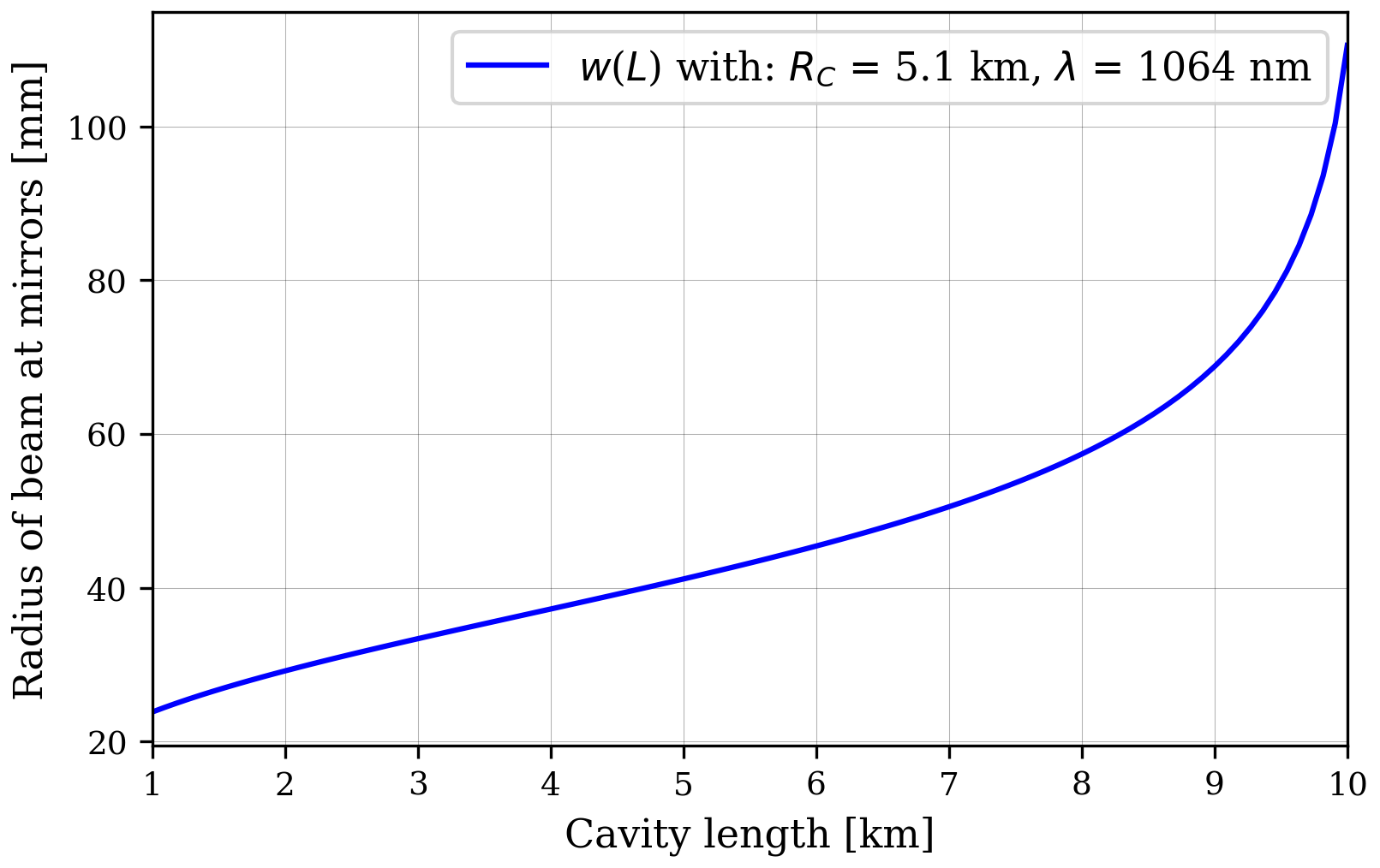
cavcalc w -L "1 10 100 km" -Rc 5.1km --plot
This results in a plot (see below) showing how the beam radius at the mirrors of a symmetric cavity varies from a cavity length of 1 km to 10 km with 100 data points, with the radii of curvature of both mirrors fixed at 5.1 km.
Alternatively one could use a file of data, e.g:
cavcalc gouy -L 5cm -w beam_radii.txt --plot --saveplot symmcav_gouy_vs_ws.png
This then computes the round-trip Gouy phase (in degrees) of a symmetric cavity of length 5cm
using beam radii data stored in a file beam_radii.txt, and plots the results (see below). Note also that
you can save the resulting figure using the --saveplot <filename> syntax as seen in the above command.
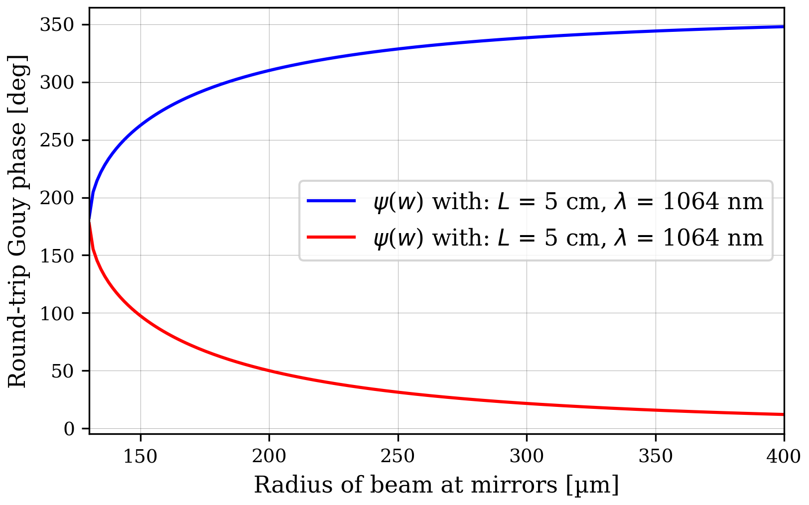
From the plot above you can also see that cavcalc supports automatically plotting of quantities which can be dual-valued. In this case, the Gouy phase can be one of two values for each beam radius; this is due to the nature of the equations which govern the Fabry-Perot cavity dynamics.
Image / density plots via --mesh
When multiple arguments are given as data-ranges, one can use the --mesh option to construct mesh-grids
of these parameters. This allows cavcalc to automatically produce image plots. For example:
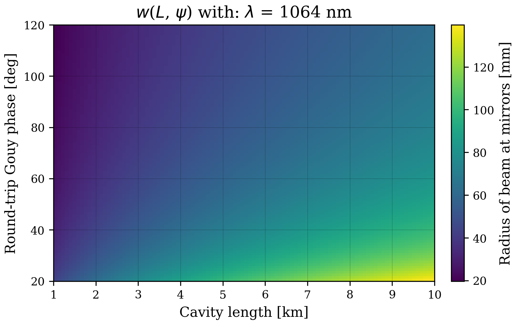
cavcalc w -L "1 10 100 km" -gouy "20 120 100 deg" --mesh true --plot
computes the radius of the beam on the mirrors of a symmetric cavity, against both the cavity length and
round-trip Gouy phase on a grid. This results in the plot shown below. Note that we simply used --mesh true
here, which automatically determines the ordering of the mesh-grid parameters based on the order in which
these parameters were given. One could replace the above with, e.g., --mesh "gouy,L" to reverse the order
of the mesh-grid; and thereby flip the parameter axes on any automated plots.
A matplotlib compliant colour-map can be specified when making an image plot using the --cmap <name> option. For example,
the following command gives the plot shown below.
cavcalc gouy -g1 "-2 2 499" -g2 g1 --mesh true --plot --cmap Spectral_r
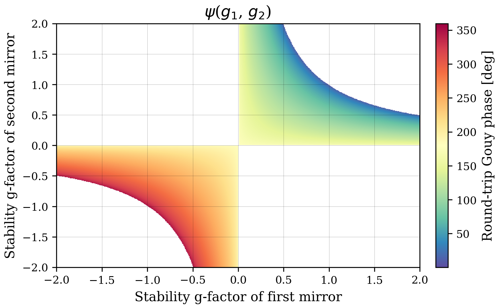
Note that here we also used the parameter-referencing feature of cavcalc, introduced in v1.2.0, to set
the values of g2 to those of g1.
A note on g-factors
Stability (g) factors are split into four different parameters for implementation purposes and to hopefully make it clearer as to which argument is being used and whether the resulting cavity computations are for a symmetric or asymmetric cavity. These arguments are detailed here:
-gs: The symmetric, singular stability factor. This represents the individual g-factors of both cavity mirrors. Use this to define a symmetric cavity where the overall cavity g-factor is then simplyg = gs * gs.-g: The overall cavity stability factor. This is the product of the individual g-factors of the cavity mirrors. Use this to define a symmetric cavity where the individual g-factors of both mirrors are thengs = +/- sqrt(g).-g1: The stability factor of the first cavity mirror. Use this to define an asymmetric cavity along with the argument-g2such that the overall cavity g-factor is theng = g1 * g2.-g2: The stability factor of the second cavity mirror. Use this to define an asymmetric cavity along with the argument-g1such that the overall cavity g-factor is theng = g1 * g2.
Using cavcalc programmatically
As well as providing a CLI, cavcalc has a full API which allows users to interact with this tool
via Python. The recommended method for doing this is to use the single-function interface via
cavcalc.calculate. This
function works similarly to the CLI, where a target can be specified along with a variable number of keyword
arguments corresponding to the physical parameters. This function then returns one of two output objects (SingleOutput
if a target was given, MultiOutput otherwise); see cavcalc.output
for details.
For example, the following script will compute all available targets from the cavity length and mirror radii of curvature provided:
import cavcalc as cc

# Specifying no target means all possible targets are computed
out = cc.calculate(L="4km", Rc1=1934, Rc2=2245)

# Printing the output object results in the same output as
# you would see when running via the CLI
print(out)
producing:
Given:
	Cavity length = 4 km

	Radius of curvature of first mirror = 1934 m
	Radius of curvature of second mirror = 2245 m

	Wavelength of beam = 1064 nm

Computed:
	FSR = 37474.05725 Hz
	Mode separation frequency = 4988.072188176178 Hz

	Position of beam waist (from first mirror) = 1837.2153886417168 m

	Radius of beam at first mirror = 53.421066433049255 mm
	Radius of beam at second mirror = 62.448079883230896 mm
	Radius of beam at waist = 11.950538458990879 mm

	Stability g-factor of cavity = 0.8350925761717987
	Stability g-factor of first mirror = -1.0682523267838677
	Stability g-factor of second mirror = -0.7817371937639199

	Round-trip Gouy phase = 312.0813565565169 deg

	Divergence angle = 0.0016237789746943276 deg
An extra feature of the API is the ability to use the cavcalc.configure function for overriding
default behaviour. For example, in the script below we use this in a context-managed scope to
temporarily use microns for any beam radius parameters, mm for distances, and GHz for any frequencies:
import cavcalc as cc

# Temporarily override units...
with cc.configure(beamsizes="um", distances="mm", frequencies="GHz"):
    out = cc.calculate(L=8, gouy=121)
    print(out)

# ... previous state (using loaded config options) will
# be restored on exit from the with block above
resulting in:
Given:
    Cavity length = 8 mm

    Round-trip Gouy phase = 121 deg

    Wavelength of beam = 1064 nm

Computed:
    FSR = 18.737028625 GHz
    Mode separation frequency = 6.297723510069445 GHz

    Position of beam waist (from first mirror) = 4.0 mm

    Radius of curvature of both mirrors = 0.01576117284251957 m

    Radius of beam at mirrors = 55.79464044247193 µm
    Radius of beam at waist = 48.19739141432035 µm

    Stability g-factor of cavity = 0.2424809625449729
    Stability g-factor of both mirrors = 0.4924235601034671

    Divergence angle = 0.40260921048107506 deg
Release history Release notifications | RSS feed


Download files
Download the file for your platform. If you're not sure which to choose, learn more about installing packages.
Source Distribution
Built Distribution
Filter files by name, interpreter, ABI, and platform.
If you're not sure about the file name format, learn more about wheel file names.
Copy a direct link to the current filters
File details
Details for the file cavcalc-1.3.0.tar.gz.
File metadata
- Download URL: cavcalc-1.3.0.tar.gz
- Upload date:
- Size: 54.4 kB
- Tags: Source
- Uploaded using Trusted Publishing? No
- Uploaded via: twine/5.1.1 CPython/3.13.0
File hashes
| Algorithm | Hash digest | |
|---|---|---|
| SHA256 |
a1e0b66912ccd6718c3e5176a00be92779984a86045da33c81627b517c4b953c
|
|
| MD5 |
ef6caa594f2e6573db00ccab8e4cadd4
|
|
| BLAKE2b-256 |
c779195e47cb4a95fd30faa9e636aedbe1d3de0289f0a898073f0b7a8fd73ec3
|
File details
Details for the file cavcalc-1.3.0-py3-none-any.whl.
File metadata
- Download URL: cavcalc-1.3.0-py3-none-any.whl
- Upload date:
- Size: 60.5 kB
- Tags: Python 3
- Uploaded using Trusted Publishing? No
- Uploaded via: twine/5.1.1 CPython/3.13.0
File hashes
| Algorithm | Hash digest | |
|---|---|---|
| SHA256 |
2721864b43650662ca72a452aa6318999f193ade5a461d3076da4d0d1a1d0687
|
|
| MD5 |
684c7e88b7012a5110264b2544992f04
|
|
| BLAKE2b-256 |
8af026811e59df50151eb611dfc040c185830dc184bd1b51755503918c2a5927
|


