chiral-transfermatrix is a transfer/scattering matrix package for calculating the optical response of achiral and chiral multilayer structures.

Project description
Introduction
chiral-transfermatrix is a Python library using the transfer matrix approach for calculating scattering properties of multilayer structures including chiral materials, and allowing for the inclusion of arbitrary optical elements (such as metamaterial mirrors) that are defined by their transfer matrix (assumed to be calculated/modeled externally).
Installation
Install the package with pip:
pip install chiral-transfermatrix
Usage
All the following examples assume that the following modules are imported:
import chiral_transfermatrix as ct
import numpy as np
import matplotlib.pyplot as plt
Simple example
An extremely simple example (a 100nm dielectric layer surrounded by air) is given by the following:
air_infty = ct.MaterialLayer(d=np.inf, eps=1, kappa=0, mu=1)
dielectric = ct.MaterialLayer(d=100., eps=2.25, kappa=0, mu=1)
layers = [air_infty, dielectric, air_infty]
lambda_vac = [800, 1200, 2400]
theta0 = 0.1*np.pi
mls = ct.MultiLayerScatt(layers, lambda_vac, theta0)
Here, the elements of layers can be either:
MaterialLayerobjects representing a uniform material layer, which are constructed with the following arguments:d: thickness of the layer (in arbitrary units, butlambda_vacmust be in the same units)eps: dielectric constant of the layerkappa: Pasteur chirality parameter of the layer (default: 0)mu: magnetic permeability of the layer (default: 1)
TransferMatrixLayerobjects representing an arbitrary optical element defined by its transfer matrix (assumed to be calculated/modeled externally), and constructed with a single argument:M: 4x4 transfer matrix of the optical element.
The "main" class is MultiLayerScatt, which calculates the scattering properties of the structure upon instantiation and takes the following arguments:
layers: list describing the layers of the structurelambda_vac: vacuum wavelength (in the same units asdabove)theta0: incidence angle (in radians)
The scattering properties can then be accessed as attributes of the returned object mls, e.g.:
> print(mls.Tsp)
[0.87296771 0.92228172 0.97604734]
Here, Tsp is the transmission (T) probability from left to right (s) for positively circular polarized light (p) at the three frequencies. The eight available scattering probabilities are: Tsp, Tsm, Tdp, Tdm, Rsp, Rsm, Rdp, Rdm, where the letters stand for:
T/R: Transmission / Reflection probabilitys/d: Light propagating from left to right (sinister) / right to left (dexter)p/m: Circularly polarized light with positive/negative helicity
The full scattering amplitudes (and not just probabilities) are also available:
> print(mls.ts)
[[[0.35434266+8.64476289e-01j 0.0066483 +6.74822883e-03j]
  [0.0066483 +6.74822883e-03j 0.35434266+8.64476289e-01j]]

 [[0.66304545+6.94690211e-01j 0.00760444+3.55144746e-04j]
  [0.00760444+3.55144746e-04j 0.66304545+6.94690211e-01j]]

 [[0.90486447+3.96546018e-01j 0.00319508-2.94518152e-03j]
  [0.00319508-2.94518152e-03j 0.90486447+3.96546018e-01j]]]
which gives the transmission/reflection (t/r) amplitudes from left to right/right to left (s/d). In the example above, these are 3×2×2 arrays, where the first index is the frequency, the second is the output polarization (in order p/m), and the third is the input polarization (same order). Since the amplitudes are not diagonal in polarization, this output is always in matrix form (the probabilities with capital letters above are summed over the output polarization).
Parameter scans
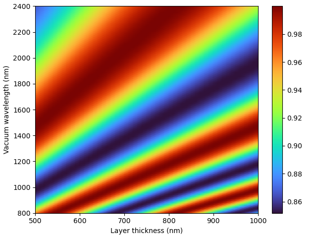
Importantly, the MultiLayerScatt interface is written to follow the numpy broadcasting conventions, so that scanning over any desired combination of parameters is easy:
# we want to scan over layer thickness d AND vacuum wavelength lambda_vac
# so make them a 51-element 1D and a 101x1 2D array, respectively,
# to give you 101x51 2D output arrays
d = np.linspace(500, 1000, 51)
lambda_vac = np.linspace(800, 2400, 101)[:,None]

air_infty = ct.MaterialLayer(d=np.inf, eps=1)
dielectric = ct.MaterialLayer(d=d, eps=2.25)
layers = [air_infty, dielectric, air_infty]
theta0 = 0.3
mls = ct.MultiLayerScatt(layers, lambda_vac, theta0)

plt.pcolormesh(d, lambda_vac, mls.Tsp, cmap='turbo', shading='gouraud')
plt.colorbar()
plt.xlabel('Layer thickness (nm)')
plt.ylabel('Vacuum wavelength (nm)')
plt.tight_layout(pad=0.5)
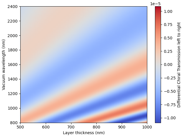
Chiral materials
We now make the dielectric material chiral, with Pasteur chirality parameter kappa=1e-3. Since this is small, the transmission for left- and right-circular polarized light are visually indistinguishable, and we instead plot the differential chiral transmission DCT = 2(Tp - Tm)/(Tp + Tm):
d = np.linspace(500, 1000, 51)
lambda_vac = np.linspace(800, 2400, 101)[:,None]

air_infty = ct.MaterialLayer(d=np.inf, eps=1)
dielectric = ct.MaterialLayer(d=d, eps=2.25, kappa=1e-3)
layers = [air_infty, dielectric, air_infty]
theta0 = 0.3
mls = ct.MultiLayerScatt(layers, lambda_vac, theta0)

vmax = abs(mls.DCTs).max()
plt.pcolormesh(d, lambda_vac, mls.DCTs, cmap='coolwarm',
               vmin=-vmax, vmax=vmax, shading='gouraud')
cb = plt.colorbar()
cb.set_label('Differential Chiral Transmission left to right')
plt.xlabel('Layer thickness (nm)')
plt.ylabel('Vacuum wavelength (nm)')
plt.tight_layout(pad=0.5)
Arbitrary layers defined by their transfer matrix
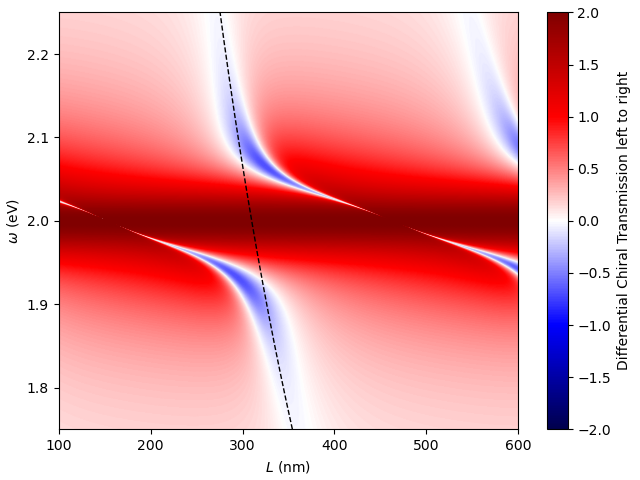
chiral-transfermatrix also supports the use of layers that are not just uniform material layers, but, e.g., metamaterials described by a transfer matrix that is externally provided. This is done by passing a TransferMatrixLayer object, which is a simple container for the transfer matrix. The transfer matrix must be passed as an ...×4×4 array, where the ... indicate an arbitrary number of dimensions that are treated according to broadcasting rules (e.g., these can describe frequency dependence), and the last two dimensions describe the transfer matrix, where the 4 entries correspond to (sp,sm,dp,dm) waves. Here again, s/d stand for left- (sinister) and right-going (dexter) waves, and p/m corresponds to a helicity of plus/minus 1 of circularly polarized light. For example, this can be used to describe a helicity-preserving mirror, and the model described in Phys. Rev. A 107, L021501 (2021) is already provided in the code with a separate helper function helicity_preserving_mirror(omegaPR,gammaPR,omega,enantiomer=False) that returns the transfer matrix for a mirror with a helicity-preserving resonance at frequency omegaPR and with linewidth gammaPR, for frequencies omega. The enantiomer argument can be used to obtain the enantiomer (i.e., mirror image) version of the mirror, as necessary for creating a helicity-preserving cavity.
The following example implements such a helicity-preserving cavity (corresponding to Fig. 3 of Phys. Rev. A 107, L021501 (2021)):
# scan over frequency omega and cavity length L (indices iomega, iL)
omega = np.linspace(1.75, 2.25, 900)[:,None]
lambda_vac = 1239.8419843320028 / omega # lambda in nm, "magic" constant is hc in eV*nm
L = np.linspace(100, 600, 1000)

mirror_1 = ct.helicity_preserving_mirror(omega,omegaPR=2,gammaPR=0.05,enantiomer=False)
mirror_2 = ct.helicity_preserving_mirror(omega,omegaPR=2,gammaPR=0.05,enantiomer=True)
air_infty = ct.MaterialLayer(d=np.inf, eps=1)
air_cav = ct.MaterialLayer(d=L, eps=1)
layers = [air_infty, mirror_1, air_cav, mirror_2, air_infty]
mls = ct.MultiLayerScatt(layers, lambda_vac, theta0=0.)

plt.pcolormesh(L, omega, mls.DCTs, cmap='seismic', vmin=-2, vmax=2, shading='gouraud')
cb = plt.colorbar()
cb.set_label('Differential Chiral Transmission left to right')
plt.xlabel(r'$L$ (nm)')
plt.ylabel(r'$\omega$ (eV)')

# line at L == lambda/2
Lcut = lambda_vac.squeeze() / 2
plt.plot(Lcut,omega.squeeze(),'k--',lw=1)
plt.tight_layout(pad=0.5)
Example notebooks
In the "examples" directory, there are two Jupyter notebooks that show how to use chiral-transfermatrix to reproduce the results published in Phys. Rev. A 108, 069902 (2023) (the erratum for Phys. Rev. A 107, L021501 (2023)), and in arXiv:2304.12140.
To do
- add example with field amplitudes
Release history Release notifications | RSS feed


Download files
Download the file for your platform. If you're not sure which to choose, learn more about installing packages.
Source Distribution
Built Distribution
Filter files by name, interpreter, ABI, and platform.
If you're not sure about the file name format, learn more about wheel file names.
Copy a direct link to the current filters
File details
Details for the file chiral_transfermatrix-0.1.2.tar.gz.
File metadata
- Download URL: chiral_transfermatrix-0.1.2.tar.gz
- Upload date:
- Size: 1.7 MB
- Tags: Source
- Uploaded using Trusted Publishing? No
- Uploaded via: python-requests/2.31.0
File hashes
| Algorithm | Hash digest | |
|---|---|---|
| SHA256 |
d29f5625781c7da173d55fdda5e207c7d024af2dc317d0e66888014d60f17c75
|
|
| MD5 |
b6ffbb348323cff878251f3dcdc89de3
|
|
| BLAKE2b-256 |
f8d8350c7775ba8df53004b3e47683f767d8f5a1f570b4e17e519d2d486cf434
|
File details
Details for the file chiral_transfermatrix-0.1.2-py3-none-any.whl.
File metadata
- Download URL: chiral_transfermatrix-0.1.2-py3-none-any.whl
- Upload date:
- Size: 9.4 kB
- Tags: Python 3
- Uploaded using Trusted Publishing? No
- Uploaded via: python-requests/2.31.0
File hashes
| Algorithm | Hash digest | |
|---|---|---|
| SHA256 |
32c82bf092922c44beee8b28cfcaaab156bee1eb9641ba277d06b70d9f1c0af1
|
|
| MD5 |
9c2c120cb24c0ed48843264fe276ee13
|
|
| BLAKE2b-256 |
3746bb51674087182cc824161d3ed44a20231936ebccaab8e446ce7c753da12a
|


