A package to calculate confidence intervals for classification positive rate, precision, NPV, and recall using a labeled sample of the population via exact & approximate Frequentist & Bayesian setups.

Project description


Classification Confidence Intervals
A package to calculate confidence intervals for classification positive rate, precision, NPV, and recall using a labeled sample of the population via exact & approximate Frequentist & Bayesian setups.
Summary
Description
Precision and recall are important metrics for evaluating classification model performance; however, they are only calculable from labeled data. In situations with unlabeled data, especially with large datasets or datastreams where labeling and remediating flagged points is incredibly expensive, exact precision and recall are not obtainable. There are solutions to calculating population precision and recall confidence intervals in such cases using a labeled sample of the entire dataset, but much of this information is scattered. This package combines Frequentist and Bayesian statistical approaches to produce various confidence intervals and present a holistic picture into model performance and dataset quality.
Metrics
The classification metrics for which confidence intervals are constructed are defined here. These metrics are also our parameters of interest in the models.
Let TP, FP, TN, FN mean true positives, false positives, true negatives, and false negatives, respectively.
- Positive Rate: (TP+FN) / (TP+FN+FP+TN)
- Precision (PPV): (TP) / (TP+FP)
- Negative Predictive Value (NPV): (TN) / (TN+FN)
- Recall (TP) / (TP+FN)
If helpful, see the precision recall image here.
Usage
The relevant class is ClassificationConfidenceIntervals.
Installation
$ pip install classification-confidence-intervals
Instantiation
During instantiation, all distributions are fitted. By default, exact_precision=None.
Args:
- sample_labels (list): Binary labels of datapoints in sample, with labels as boolean or binary in [0,1] or in [-1,1].
- sample_predictions (list): Binary labels of datapoints in sample flagged as positives by algorithm, with labels as boolean or binary in [0,1] or in [-1,1].
- population_size (int): Size of population.
- population_flagged_count, (int): Number of datapoints in population flagged as positives by algorithm.
- confidence_level (float): Confidence level, equal to area desired under curve.
- exact_precision (float): If provided, the actual population precision.
>>> from classificationconfidenceintervals import ClassificationConfidenceIntervals
>>> confidenceintervals = ClassificationConfidenceIntervals(
...     sample_labels=[1, 1, 1, 0, 0, 0, 0, 0] * 30,
...     sample_predictions=[1, 1, 0, 0, 1, 1, 0, 0] * 30,
...     population_size=4000,
...     population_flagged_count=2000,
...     confidence_level=0.95,
... )
With regards to your labled sample, in the example above using fake labels and predictions, sample_labels refer to the truth values of each datapoint (the 1st to 3rd datapoint are positives; the 4th to 8th datapoints are negatives). sample_predictions refer to whether or not your algorithm flagged each datapoint (the 1st, 2nd, 5th, and 6th datapoints were flagged; the 3rd, 4th, 7th, and 8th datapoints were not flagged). The arrays are artificially duplicated by a factor of 30 in the example. Do not do this in practice.
With regards to your population, the only information required are population_size and how many points your algorithm flags in the population as population_flagged_count. In the example above, and the algorithm flagged 2000 datapoints among the 4000 datapoints in the population.
Degenerate samples cause the models to become degenerate, and instantiation will throw errors if your sample does not include at least one of each of TP, FP, TN, FN.
confidence_level by convention should generally be set at .95. The higher the value, the wider the confidence intervals.
In cases where all flagged datapoints in the population have been remediated (i.e. are labeled), you may provide the exact_precision value during instantiation; otherwise, confidence intervals will also be created for precision. A case where not all flagged datapoints in the population are remediated is when the total number of flagged items is simply too large and only a subset of them have been remediated.
Your sample size should be sufficiently large to make the confidence intervals narrow. See the appendix below.
Getting Confidence Intervals
After instantiation, calculations for confidence intervals can now be performed via the get_cis() method. By default, n_iters=1000000 and plot_filename is an empty string.
Args:
- n_iters (int): Number of iterations to simulate posterior models.
- plot_filename (str): If not empty, save plots using filename as relative path.
Returns:
- pos_rate_cis (CIDataClass): Confidence intervals for pos rate based on multiple methods.
- ppv_cis (CIDataClass): Confidence intervals for precision based on multiple methods.
- npv_cis (CIDataClass): Confidence intervals for NPV based on multiple methods.
- recall_cis (CIDataClass): Confidence intervals for recall based on multiple methods.
>>> pos_rate_cis, ppv_cis, npv_cis, recall_cis = confidenceintervals.get_cis(n_iters=100000, plot_filename='example_metrics_plot')
>>> print(pos_rate_cis)
read_only_properties.<locals>.class_rebuilder.<locals>.CustomClass(tnorm_ci=(0.31375112548312334, 0.43624887451687666), poisson_ci=(0.3, 0.45416666666666666), lrt_ci=(0.3154, 0.4373), score_ci=(0.3162, 0.43770000000000003), posterior_ci=(0.3155447558316776, 0.4374497740783102), simulated_ci=(0.3159835357403228, 0.4374219880675257))
>>> print(ppv_cis)
read_only_properties.<locals>.class_rebuilder.<locals>.CustomClass(tnorm_ci=(0.41054029281414217, 0.5894597071858578), poisson_ci=(0.375, 0.6333333333333333), lrt_ci=(0.4113, 0.5887), score_ci=(0.41200000000000003, 0.588), posterior_ci=(0.41143373746262163, 0.5885662625373784), simulated_ci=(0.4119916854809507, 0.5890112681445884))
>>> print(npv_cis)
read_only_properties.<locals>.class_rebuilder.<locals>.CustomClass(tnorm_ci=(0.6725256210456648, 0.8274743790402173), poisson_ci=(0.6, 0.9083333333333333), lrt_ci=(0.6678000000000001, 0.8216), score_ci=(0.6656, 0.8189000000000001), posterior_ci=(0.667214568760124, 0.8208930781209349), simulated_ci=(0.6675875145345339, 0.8210540703047337))
>>> print(recall_cis)
read_only_properties.<locals>.class_rebuilder.<locals>.CustomClass(tnorm_ci=(0.5562766006133449, 0.7735840644338399), poisson_ci=(0.4838709677419355, 0.8735632183908046), lrt_ci=(0.5531943510423672, 0.767435797158128), score_ci=(0.5519828510182208, 0.7645299700949162), posterior_ci=(0.5528394789668374, 0.7666885785320019), simulated_ci=(0.5856829486565244, 0.7438937436565682))
The CIDataClass is a modified class that supports dot notation access and forces the returned confidence intervals to be read-only.
>>> print(pos_rate_cis.tnorm_ci)
(0.31375112548312334, 0.43624887451687666)
>>> pos_rate_cis.tnorm_ci = tuple([.5, .8])
AttributeError: Can't modify tnorm_ci
For variable access, a get() method is provided as well in CIDataClass.
>>> key = "tnorm_ci"
>>> print(pos_rate_cis.get(key))
(0.31375112548312334, 0.43624887451687666)
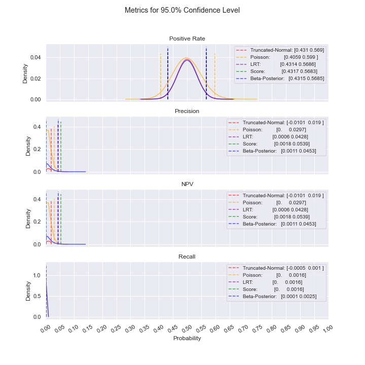
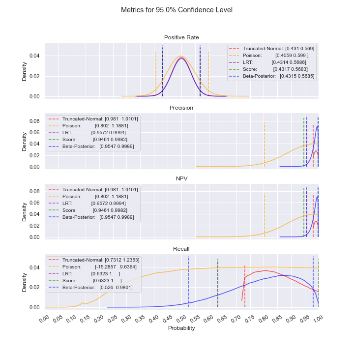
Visualization
If plot_filename is not an empty string when running get_cis(), you will have an image file located at plot_filename.png. An example is provided below.

Interpretation
Let p be the probability for a metric. There are three cases to consider.
-
p is not close to 0 nor 1: Ensure that the non-Poisson confidence intervals are similar before using any of the non-Poisson confidence intervals (as they are all similar).
- If non-Poisson confidence intervals are not similar, then include more labeled samples as inputs to the class. This helps to ensures that all non-Poisson methods agree asymptotically on the confidence intervals.
-
p is close to 0: Use the Poisson confidence intervals.
- Increasing the labeled sample size does not necessarily ensure that non-Poisson models will agree asymptotically on what the confidence intervals should be. See the appendix for more details.
-
p is close to 1: Use one of the non-Truncated-Normal/non-Poisson confidence intervals.
- Increasing the labeled sample size does not necessarily ensure that non-Truncated-Normal/non-Poisson models will agree asymptotically on what the confidence intervals should be. See the appendix for more details.
Models
For the four metrics of interest, the following models are used. Please note that all models are fitted for Positive Rate, Precision, and NPV. The only model used for Recall is the Simulated Distribution. As discussed below, no parametric distributions can be fit on recall due to independence constraints for calculating confidence intervals.
Frequentist Models:
Exact distribution:
The exact underlying model fits the story of a binomial distribution. From some total sample size, each item in that sample has some probability of being a success or a failure.
- Binomial: Binomial distribution.
Approximating distribution:
These models approximate the exact binomial distribution as the sample size grows.
- Truncated-Normal: A normal distribution truncated to (0, 1). Theoretically preferred if the estimate for the parameter is not close to 0 nor 1.
- Poisson: Poisson distribution. Theoretically preferred if the estimate for the parameter is close to 0.
Bayesian Models
Exact distribution:
While Frequentist statistics view estimates for the parameter as completely determined by observed data, Bayesian statistics models the parameter with a prior belief via a distribution that causes the parameter to depend on both the prior belief and the observed data. A flat prior of Beta(.5,.5) is used in this package.
- Beta-Posterior: A Beta-Posterior distribution with the Beta distribution as the conjugate prior to the Binomial distribution.
Approximating distribution:
This model approximates the Beta-Posterior distribution as the number of Monte Carlo draws grows.
- Simulated Distribution: A non-parametric distribution created from Monte Carlo samples from the Beta-Posterior distribution.
Confidence Interval Methods
The models above are used to obtain confidence intervals for each of the metrics in three ways. For ease of discussion, confidence intervals also refer to credible intervals under the Bayesian framework. This section focuses on derivations, not proofs, the latter of which are readily available at online sources.
Distributional Confidence Intervals (Truncated-Normal, Poisson, Beta-Posterior)
Positive Rate, Precision, and NPV
Given c=confidence_level, confidence intervals are drawn from the quantiles of the model's probability mass/density function such that the center (confidence_level)% of area lies within the confidence interval.
For the Poisson model, an extra adjustment is performed. The support represents the count of successes and is divided by the model's relevant sample size to map to proportions;
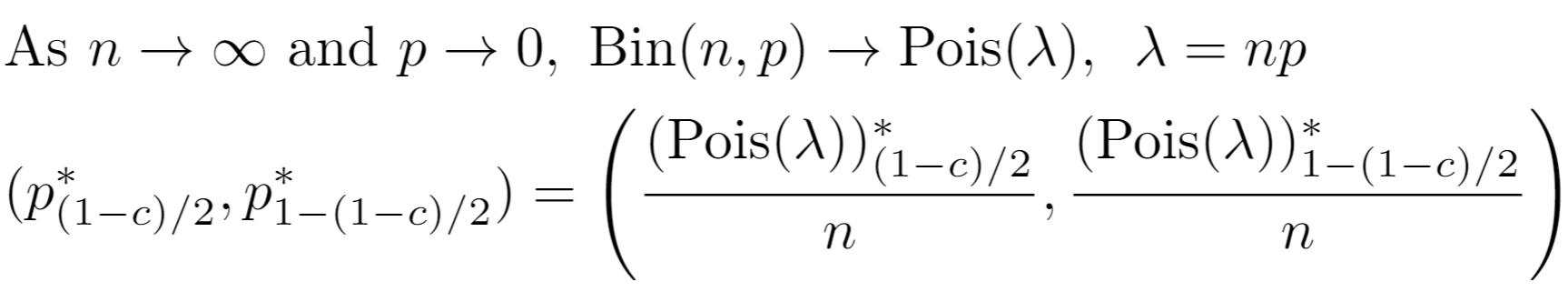
Recall
For recall, let Xm be the precision distribution under model m and Ym be the NPV distribution under model m. Let N be the population size. Let Nf be number of datapoints in population flagged as positives by the algorithm. Then, for model m, the population recall is Xm Nf / (Xm Nf + Ym (N-Nf)).
There is no clean distributional form for recall due to dependence between the numerator and denominator, but the confidence interval for recall is obtainable by optimizing for the endpoints of the confidence interval for recall using Xm and Ym. Let Xm,l and Xm,h be the respective lower and upper bounds of the confidence interval for Xm. Then the confidence intervals for population recall are:

Independence between Xm and Ym grants the ability to use each each distribution's confidence intervals without concern for dependence effects. Had recall been defined as precision / positives, the parameters of the two distributions are not independent and confidence intervals could not be created in the above manner.
Hypothesis Test Inversion Confidence Intervals (Binomial)
Positive Rate, Precision, and NPV
Confidence intervals are created by inverting the Binomial Likelihood Ratio Test (LRT) and Score Test. Considering only the parameter values for where the test statistic does not lie in the rejection region determined by confidence_level, we take the min and max of those values to get confidence intervals.
Let n be the number of observations and y be the number of successes. The binomial loglikelihood and score function are respectively defined as:
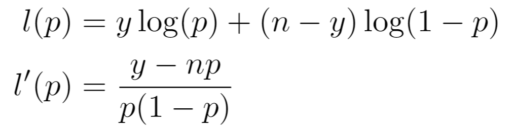
Then the LR test statistic and Score test statistic respectively are:
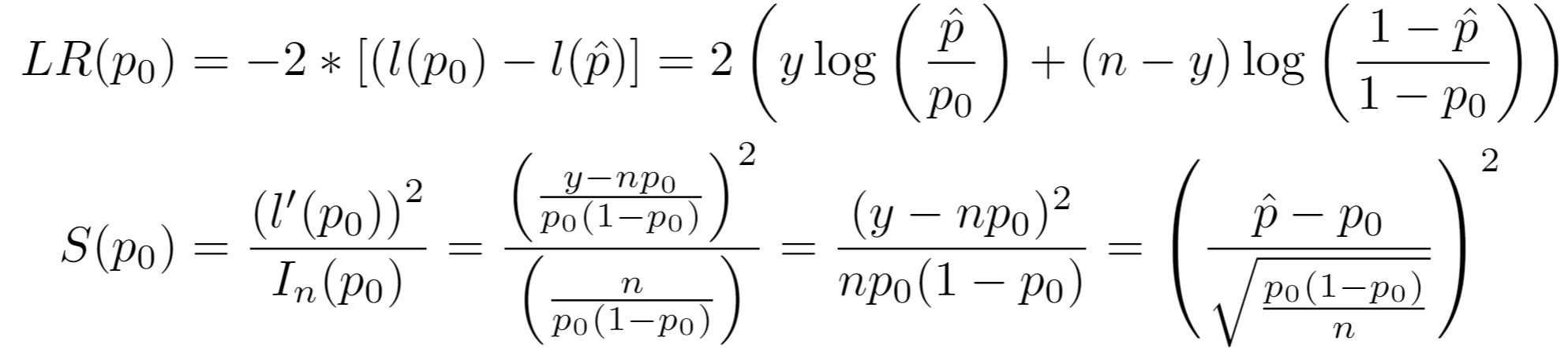
Under the null hypothesis:
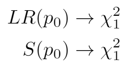
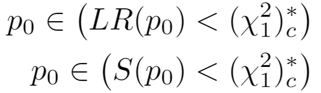
Invoking a one-sided test on the chi-squared distribution letting c = confidence_level, the confidence intervals for the LRT and Score Test are respectively given by taking the min and max of:
Recall
For recall, the same logic follows as for distributional confidence intervals.
Simulated Confidence Intervals (Simulated)
Positive Rate, Precision, and NPV
Given confidence_level, confidence intervals are drawn from the quantiles of the Monte Carlo simulated draws from the Beta-Posterior such that the center (confidence_level)% of area lies within the confidence interval.
Recall
For recall, let p|X be the Beta-Posterior distribution for precision, where X is the observed binary labeled data, as such:
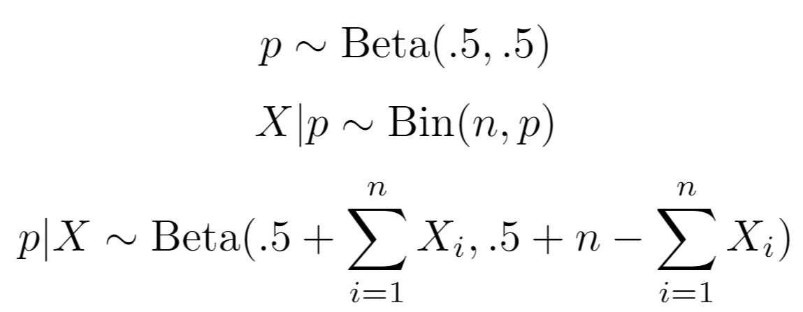
Let p|Y similarly be the Beta-Posterior distribution for NPV.
Let R(i) be the i'th Monte Carlo sample value for population recall. Let N be the population size. Let Nf be number of datapoints in population flagged as positives by the algorithm. Then, based on the independent draws for p|X and p|Y on the i'th iteration:
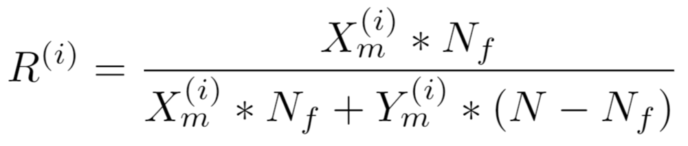
from which quantiles are drawn.
Appendix
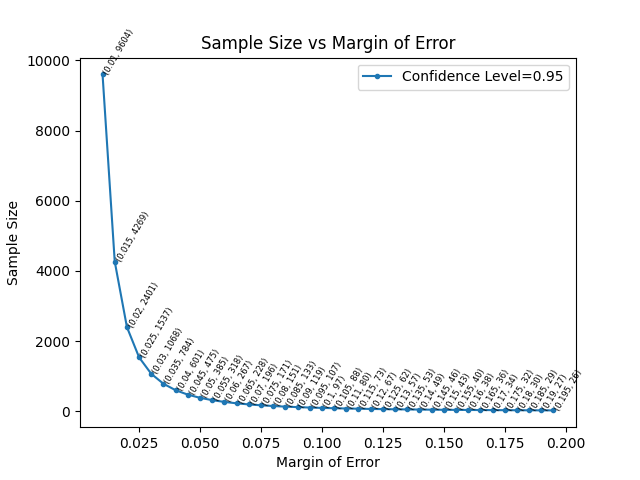
Sample Size and Margin of Error
Under the convention of confidence_level=.95, the plot below shows the necessary sample size for a particular proportion to have a certain margin of error under a Wald confidence interval (Normal model). Margin of error gives the number of percentage points (on a decimal scale) from the estimate of the proportion to the confidence interval endpoint on either side of the estimate.
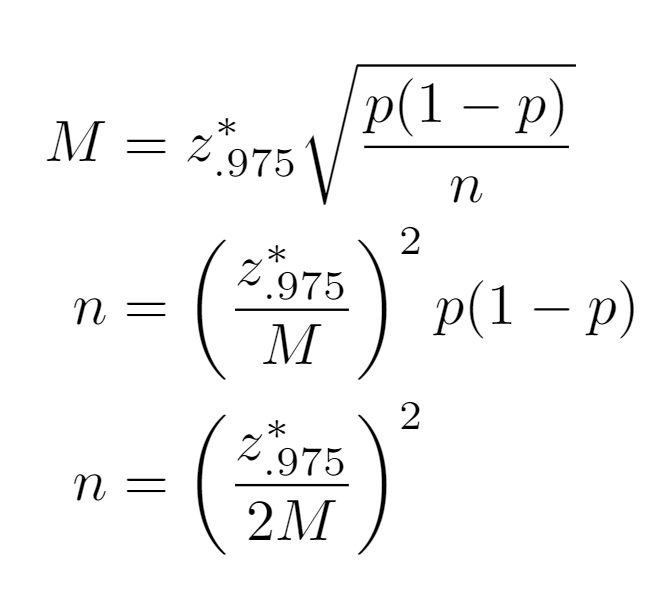
With a desired Margin of Error M, one can invert the equation for the spread in a Wald confidence interval to solve for sample size n. Since the true parameter p is unknown, to be conservative and maximize the required sample size, p is set to .5.
Examples of Extreme Values of p
>>> # estimate near 0
>>> for n in [10, 100]:
...     module = ClassificationConfidenceIntervals(
...         sample_labels=[0] * n + [1] + [1] * n + [0],
...         sample_predictions=[1] * (n + 1) + [0] * (n + 1),
...         population_size=4000,
...         population_flagged_count=200,
...         confidence_level=0.95,
...     )
...     module.get_cis(plot_filename=f"near_0_n={n}")

>>> # estimate near 1
>>> for n in [10, 100]:
...     module = ClassificationConfidenceIntervals(
...         sample_labels=[1] * n + [0] + [0] * n + [1],
...         sample_predictions=[1] * (n + 1) + [0] * (n + 1),
...         population_size=4000,
...         population_flagged_count=200,
...         confidence_level=0.95,
...     )
...     module.get_cis(plot_filename=f"near_1_n={n}")
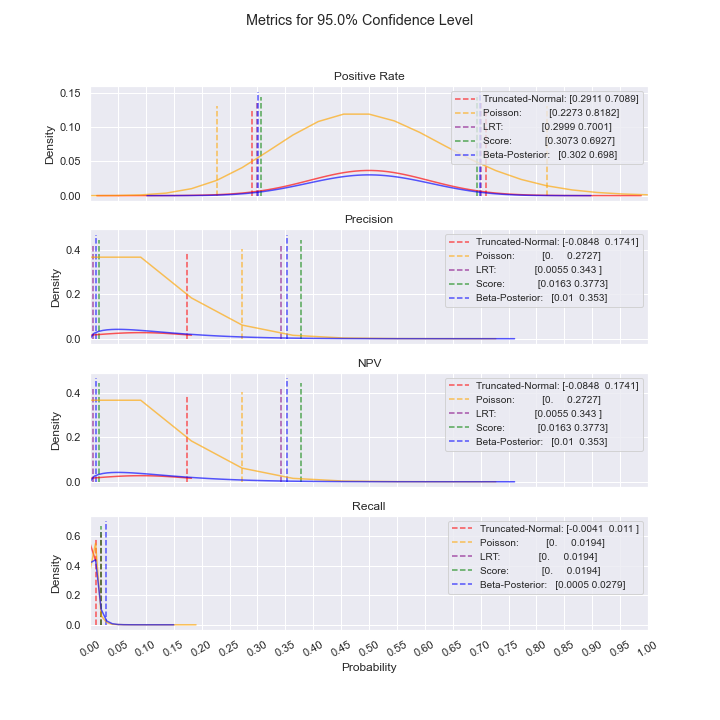
For the case above where precision and NPV are low, notice how the Truncated-Normal confidence intervals include negative values, rendering Truncated-Normal unusable in this situation. Even as sample size increases, this issue persists; additionally, we do not see convergence of the confidence intervals. As such, the best model to use is Poisson.
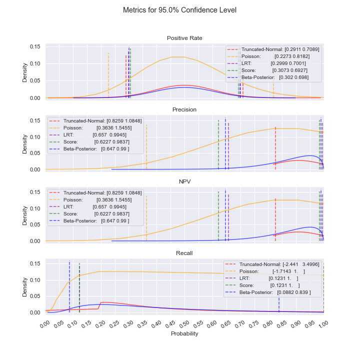
For the case above where precision and NPV are high, notice how the Truncated-Normal and Poisson confidence intervals include values above 1, rendering them unusable in this situation. Even as sample size increases, this issue persists; additionally, we do not see convergence of the confidence intervals. As such, one of the other models should be used (LRT or Bayesian).
Comparison of Wald, LRT, and Score Confidence Intervals
- Wald (Truncated-Normal): Inflates Type I error because standard error is calculated under the alternative.
- LRT (Binomial): Conserves Type I error and power.
- Score (Binomial): Less powerful than LRT but more robust than Wald.
Generally, LRT is the best choice among Frequentist confidence intervals.
Release history Release notifications | RSS feed


Download files
Download the file for your platform. If you're not sure which to choose, learn more about installing packages.
Source Distribution
Built Distribution
Filter files by name, interpreter, ABI, and platform.
If you're not sure about the file name format, learn more about wheel file names.
Copy a direct link to the current filters
File details
Details for the file classification-confidence-intervals-1.0.2.tar.gz.
File metadata
- Download URL: classification-confidence-intervals-1.0.2.tar.gz
- Upload date:
- Size: 10.6 kB
- Tags: Source
- Uploaded using Trusted Publishing? No
- Uploaded via: twine/3.2.0 pkginfo/1.5.0.1 requests/2.24.0 setuptools/40.8.0 requests-toolbelt/0.9.1 tqdm/4.48.0 CPython/3.7.1
File hashes
| Algorithm | Hash digest | |
|---|---|---|
| SHA256 |
d1eb043cdf49ad5e4418f56bb609dff192adecdfc1eb01bed55eac98407d9577
|
|
| MD5 |
6cc685d8efbad3376ddc827935e9874a
|
|
| BLAKE2b-256 |
76ab989cc088051dc137d9f9bc2d13a9235af7a2d849fe8a23db731ffa1f4d8f
|
File details
Details for the file classification_confidence_intervals-1.0.2-py3-none-any.whl.
File metadata
- Download URL: classification_confidence_intervals-1.0.2-py3-none-any.whl
- Upload date:
- Size: 8.5 kB
- Tags: Python 3
- Uploaded using Trusted Publishing? No
- Uploaded via: twine/3.2.0 pkginfo/1.5.0.1 requests/2.24.0 setuptools/40.8.0 requests-toolbelt/0.9.1 tqdm/4.48.0 CPython/3.7.1
File hashes
| Algorithm | Hash digest | |
|---|---|---|
| SHA256 |
bc76e2537fb38be3dc6ae873e63f877bcc9ef9532e9111263de1952bde3d5a39
|
|
| MD5 |
0c5f2374e9cde87369835c7cb7a25b7b
|
|
| BLAKE2b-256 |
922373a094d5accd86c23af8e7880104f13df4968ce8c0fef9b547e4e9b60900
|


