Consensus NMF for scRNA-Seq data


Project description
Consensus NMF (cNMF)
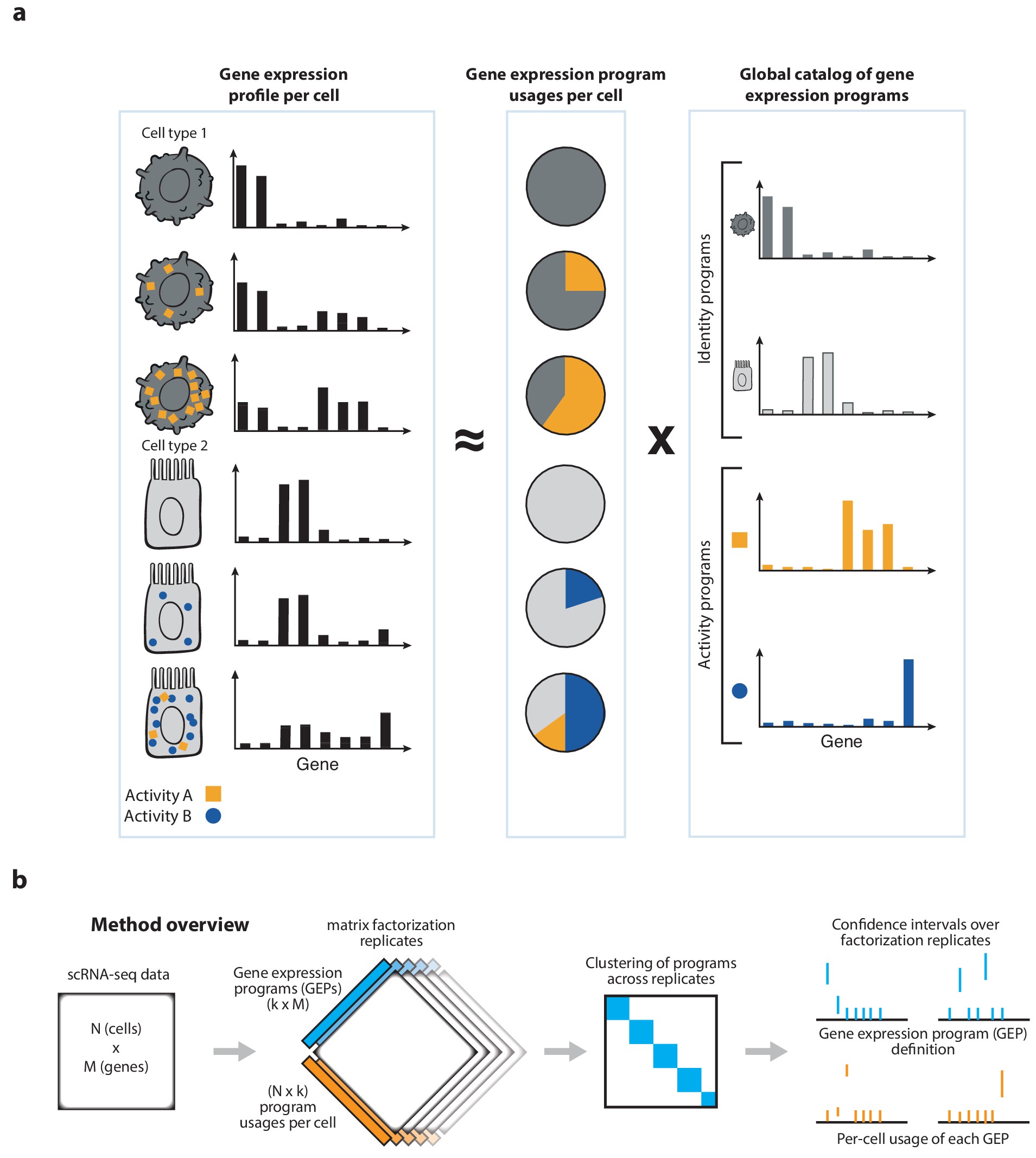
cNMF is a pipeline for inferring gene expression programs from scRNA-Seq. It takes a count matrix (N cells X G genes) as input and produces a (K x G) matrix of gene expression programs (GEPs) and a (N x K) matrix specifying the usage of each program for each cell in the data. Read more about the method in the publication and check out examples on simulated data and PBMCs.
We have also created a tutorial for running cNMF from R. See the Rmd notebook or the compiled html for this.
Installation
cNMF has been tested with Python 3.7 and 3.10 and requires scikit-learn>=1.0, scanpy>=1.8, and AnnData>=0.9
You can install with pip:
pip install cnmf
If you want to use the batch correction preprocessing, you also need to install the Python implementation of Harmony and scikit-misc
pip install harmonypy
pip install scikit-misc
Running cNMF
cNMF can be run from the command line without any parallelization using the example commands below:
cnmf prepare --output-dir ./example_data --name example_cNMF -c ./example_data/counts_prefiltered.txt -k 5 6 7 8 9 10 11 12 13 --n-iter 100 --seed 14

cnmf factorize --output-dir ./example_data --name example_cNMF --worker-index 0 --total-workers 1

cnmf combine --output-dir ./example_data --name example_cNMF

cnmf k_selection_plot --output-dir ./example_data --name example_cNMF

cnmf consensus --output-dir ./example_data --name example_cNMF --components 10 --local-density-threshold 0.01 --show-clustering
Or alternatively, the same steps can be run from within a Python environment using the commands below:
from cnmf import cNMF
cnmf_obj = cNMF(output_dir="./example_data", name="example_cNMF")
cnmf_obj.prepare(counts_fn="./example_data/counts_prefiltered.txt", components=np.arange(5,14), n_iter=100, seed=14)
cnmf_obj.factorize(worker_i=0, total_workers=1)
cnmf_obj.combine()
cnmf_obj.k_selection_plot()
cnmf_obj.consensus(k=10, density_threshold=0.01)
usage, spectra_scores, spectra_tpm, top_genes = cnmf_obj.load_results(K=10, density_threshold=0.01)
For the Python environment approach, usage will contain the usage matrix with each cell normalized to sum to 1. spectra_scores contains the gene_spectra_scores output (aka Z-score unit gene expression matrix), spectra_tpm contains the GEP spectra in units of TPM and top_genes contains an ordered list of the top 100 associated genes for each program.
Output data files will all be available in the ./example_data/example_cNMF directory including:
- Z-score unit gene expression program matrix -
example_data/example_cNMF/example_cNMF.gene_spectra_score.k_10.dt_0_01.txt - TPM unit gene expression program matrix -
example_data/example_cNMF/example_cNMF.gene_spectra_tpm.k_10.dt_0_01.txt - Usage matrix -
example_data/example_cNMF/example_cNMF.usages.k_10.dt_0_01.consensus.txt - K selection plot -
example_data/example_cNMF/example_cNMF.k_selection.png - Clustergram diagnostic plot -
example_data/example_cNMF/example_cNMF.clustering.k_10.dt_0_01.pdf
Some usage notes:
- Parallelization: The factorize step can be parallelized with the --total-workers flag and then submitting multiple jobs, one per worker, indexed starting by 0. For example:
cnmf factorize --output-dir ./example_data --name example_cNMF --worker-index 0 --total-workers 3 &
cnmf factorize --output-dir ./example_data --name example_cNMF --worker-index 1 --total-workers 3 &
cnmf factorize --output-dir ./example_data --name example_cNMF --worker-index 2 --total-workers 3 &
would break the factorization jobs up into 3 batches and submit them independently. This can be used with compute clusters to run the factorizations in parallel (see tutorials for example).
- Input data: Input data can be provided in 3 ways:
-
- as a scanpy file ending in .h5ad containg counts as the data feature. See the PBMC dataset tutorial for an example of how to generate the Scanpy object from the data provided by 10X. Because Scanpy uses sparse matrices by default, the .h5ad data structure can take up much less memory than the raw counts matrix and can be much faster to load.
-
- as a raw tab-delimited text file containing row labels with cell IDs (barcodes) and column labels as gene IDs
-
- as a 10x-Genomics-formatted mtx directory. You provide the path to the counts.mtx file or counts.mtx.gz file to counts_fn. It expects there to be barcodes.tsv and genes.tsv in the directory as well
-
See the tutorials or Stepwise_Guide.md for more details
Integration of technical variables and batches
We have implemented a pipeline to integrate batch variables prior to running cNMF and to handle ADTs in CITE-Seq. It uses an adaptation of Harmony that corrects the underlying count matrix rather than principal components. We describe it in our recent preprint. See the batch correction tutorial as well for an example.
We use a separate Preprocess class to run batch correction. You pass in an AnnData object, as well as harmony_vars, a list of the names of variables to correct correspond to columns in the AnnData obs attribute. You also specify an output file base name to save the results to like below:
from cnmf import cNMF, Preprocess
#Initialize the Preprocess object
p = Preprocess(random_seed=14)

#Batch correct the data and save the corrected high-variance gene data to adata_c, and the TPM normalized data to adata_tpm
(adata_c, adata_tpm, hvgs) = p.preprocess_for_cnmf(adata, harmony_vars=['Sex', 'Sample'], n_top_rna_genes = 2000, librarysize_targetsum= 1e6,
                                                    save_output_base='./example_islets/batchcorrect_example_sex')

#Then run cNMF passing in the corrected counts file, tpm_fn, and HVGs as inputs
cnmf_obj_corrected = cNMF(output_dir='./example_islets', name='BatchCorrected')
cnmf_obj_corrected.prepare(counts_fn='./example_islets/batchcorrect_example.Corrected.HVG.Varnorm.h5ad',
                           tpm_fn='./example_islets/batchcorrect_example.TP10K.h5ad',
                           genes_file='./example_islets/batchcorrect_example.Corrected.HVGs.txt',
                           components=[15], n_iter=20, seed=14, num_highvar_genes=2000)

#Then proceed with the rest of cNMF as normal
Change log
New in version 1.7
- Use scipy hierachical clsutering grather than fastcluster for compatibility with numpy>2.0
- More efficient sparse + batched OLS computation uses significantly less memory
- Implemented basic testing suite
New in version 1.6
- Added option in consensus() to build spectra for annotating new datasets with GEPs using starCAT.
- Added option to factorize() to skip tasks that have already completed.
New in version 1.5
- Fixed bug in detecting and printing cells with 0 counts of overdispersed genes
- Added option in load_results() to return normalized or unnormalized usage.
- Added a Preprocess class to batch correct data prior to cNMF. See the added Tutorial analyze_batcheffectcorrect_BaronEtAl.ipynb to illustrate its basic usage.
- Now accepts 10x formatted .mtx directories (containing counts.mtx, barcodes.tsv, and genes.tsv files)
New in version 1.4
- Usage is re-fit a final time from gene_spectra_tpm which increases accuracy in simulations
- Use cnmf_obj.load_results(K=, density_threshold=) to obtain usage, spectra_scores, spectra_tpm, and top_genes matrices
- cnmf_obj.combine() now has a skip_missing_files=True/False option to skip incomplete factorize iterations
- GEPs are now ordered by maximum total usage
- Now detects and errors when 0 counts of HVGs with interpretable error message
New in version 1.3
- Installation via pip
- Object oriented interface for Python users and command line script option via
cnmf
New in version 1.2
- Increased the threshold for ignoring genes with low mean expression for determining high-variance genes from a TPM of 0.01 to 0.5. Some users were identifying uninterpretable programs with very low usage except in a tiny number of cells. We suspect that this was due to including genes as high-variance that are detected in a small number of cells. This change in the default parameter will help offset that problem in most cases.
- Updated import of NMF for compatibility with scikit-learn versions >22
- Colorbar for heatmaps included with consensus matrix plot
New in version 1.1
- Now operates by default on sparse matrices. Use --densify option in prepare step if data is not sparse
- Now takes Scanpy AnnData object files (.h5ad) as input
- Now has option to use KL divergence beta_loss instead of Frobenius. Frobenius is the default because it is much faster.
- Includes a Docker file for creating a Docker container to run cNMF in parallel with cloud compute
- Includes a tutorial on a simple PBMC dataset
- Other minor fixes
Release history Release notifications | RSS feed


Download files
Download the file for your platform. If you're not sure which to choose, learn more about installing packages.
Source Distribution
Built Distribution
Filter files by name, interpreter, ABI, and platform.
If you're not sure about the file name format, learn more about wheel file names.
Copy a direct link to the current filters
File details
Details for the file cnmf-1.7.1.tar.gz.
File metadata
- Download URL: cnmf-1.7.1.tar.gz
- Upload date:
- Size: 32.4 kB
- Tags: Source
- Uploaded using Trusted Publishing? No
- Uploaded via: twine/6.2.0 CPython/3.10.19
File hashes
| Algorithm | Hash digest | |
|---|---|---|
| SHA256 |
0cbf42009399106874aafc888331baa811b129c12119bb942a23e885575e46a4
|
|
| MD5 |
66a24dd902447d93cf385d4a0f96c8c8
|
|
| BLAKE2b-256 |
ef1741f8db9080117fe5ee861fad86c9a5d0eee52d69d1b21f838c3665762de4
|
File details
Details for the file cnmf-1.7.1-py3-none-any.whl.
File metadata
- Download URL: cnmf-1.7.1-py3-none-any.whl
- Upload date:
- Size: 26.5 kB
- Tags: Python 3
- Uploaded using Trusted Publishing? No
- Uploaded via: twine/6.2.0 CPython/3.10.19
File hashes
| Algorithm | Hash digest | |
|---|---|---|
| SHA256 |
a4b237169626f632fee04a31441365669b12a02c72a93b079686b0ce47a29ec9
|
|
| MD5 |
96da6bb059ee66d7217d3ac09655880e
|
|
| BLAKE2b-256 |
b550ddd4e791070b3f6f2d072f191639d0462906d058b8f5b18a271a6395094d
|


