





The dagma library is a Python 3 package for learning DAGs (a.k.a. Bayesian networks) from data.
DAGMA works by optimizing a given score/loss function, where the structure that relates the variables is constrained to be a directed acyclic graph (DAG). Due to the super-exponential number of DAGs w.r.t. the number of variables, the vanilla formulation results in a hard combinatorial optimization problem. DAGMA reformulates this optimization problem, by replacing the combinatorial constraint with a non-convex differentiable function that exactly characterizes DAGs, thus, making the optimization amenable to continuous optimization methods such as gradient descent.
Citation
This is an implementation of the following paper:
[1] Bello K., Aragam B., Ravikumar P. (2022). DAGMA: Learning DAGs via M-matrices and a Log-Determinant Acyclicity Characterization. NeurIPS'22.
If you find this code useful, please consider citing:
BibTeX
@inproceedings{bello2022dagma,
    author = {Bello, Kevin and Aragam, Bryon and Ravikumar, Pradeep},
    booktitle = {Advances in Neural Information Processing Systems},
    title = {{DAGMA: Learning DAGs via M-matrices and a Log-Determinant Acyclicity Characterization}},
    year = {2022}
}
Features
- Supports continuous data for linear (see dagma.linear) and nonlinear models (see dagma.nonlinear).
- Supports binary (0/1) data for generalized linear models, via dagma.linear.DagmaLinear and using
logisticas score. - Faster than other continuous optimization methods for structure learning, e.g., NOTEARS, GOLEM.
Getting Started
Install the package
We recommend using a virtual environment via virtualenv or conda, and use pip to install the dagma package.
$ pip install dagma
Using dagma
See an example on how to use dagma in this iPython notebook.
An Overview of DAGMA
We propose a new acyclicity characterization of DAGs via a log-det function for learning DAGs from observational data. Similar to previously proposed acyclicity functions (e.g. NOTEARS), our characterization is also exact and differentiable. However, when compared to existing characterizations, our log-det function: (1) Is better at detecting large cycles; (2) Has better-behaved gradients; and (3) Its runtime is in practice about an order of magnitude faster. These advantages of our log-det formulation, together with a path-following scheme, lead to significant improvements in structure accuracy (e.g. SHD).
The log-det acyclicity characterization
Let $W \in \mathbb{R}^{d\times d}$ be a weighted adjacency matrix of a graph of $d$ nodes, the log-det function takes the following form:
$$h^{s}(W) = -\log \det (sI-W\circ W) + d \log s,$$
where $I$ is the identity matrix, $s$ is a given scalar (e.g., 1), and $\circ$ denotes the element-wise Hadamard product. Of particular interest, we have that $h(W) = 0$ if and only if $W$ represents a DAG, and when the domain of $h$ is the set of M-matrices then $h$ is well-defined and non-negative. For more properties of $h(W)$ (e.g., being an invex function), $\nabla h(W)$, and $\nabla^2 h(W)$, we invite you to look at [1].
A path-following approach
Given the exact differentiable characterization of a DAG, we are interested in solving the following optimization problem:
\begin{array}{cl}
\min _{W \in \mathbb{R}^{d \times d}} & Q(W;\mathbf{X}) \\
\text { subject to } & h^{s}(W) = 0,
\end{array}
where $Q$ is a given score function (e.g., square loss) that depends on $W$ and the dataset $\mathbf{X}$. To solve the above constrained problem, we propose a path-following approach where we solve a few of the following unconstrained problems:
\hat{W}^{(t+1)} = \arg\min_{W}\; \mu^{(t)} Q(W;\mathbf{X}) + h(W),
where $\mu^{(t)} \to 0$ as $t$ increases. Leveraging the properties of $h$, we show that, at the limit, the solution is a DAG. The trick to make this work is to use the previous solution as a starting point when solving the current unconstrained problem, as usually done in interior-point algorithms. Finally, we use a simple accelerated gradient descent method to solve each unconstrained problem.
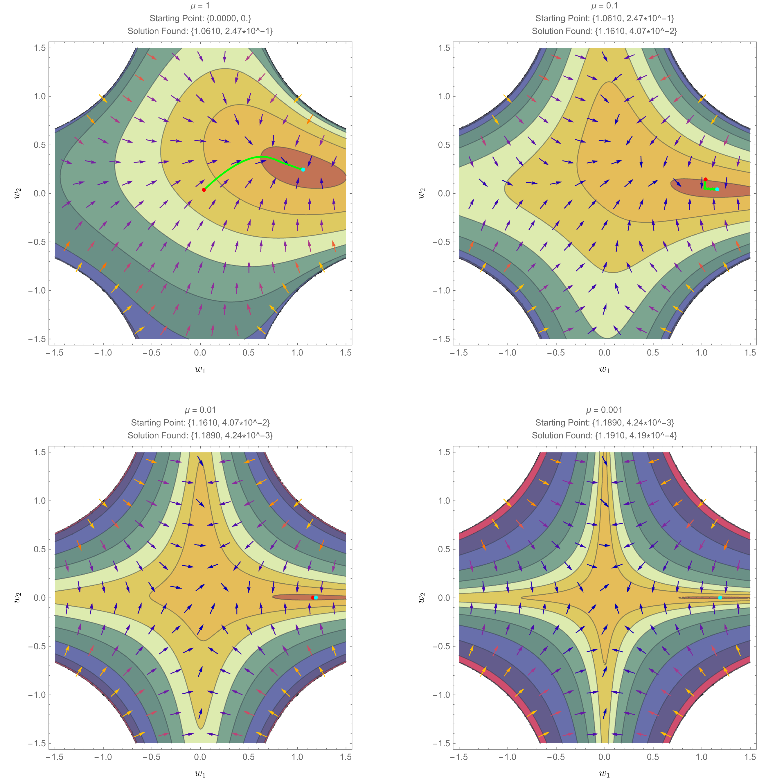
Let us give an illustration of how DAGMA works in a two-node graph (see Figure 1 in [1] for more details). Here $w_1$ (the x-axis) represents the edge weight from node 1 to node 2; while $w_2$ (y-axis) represents the edge weight from node 2 to node 1. Moreover, in this example, the ground-truth DAG corresponds to $w_1 = 1.2$ and $w_2 = 0$.
Below we have 4 plots, where each illustrates the solution to an unconstrained problem for different values of $\mu$. In the top-left plot, we have $\mu=1$, and we solve the unconstrained problem starting at the empty graph (i.e., $w_1 = w_2 = 0$), which corresponds to the red point, and after running gradient descent, we arrive at the cyan point (i.e., $w_1 = 1.06, w_2 = 0.24$). Then, for the next unconstrained problem in the top-right plot, we have $\mu = 0.1$, and we initialize gradient descent at the previous solution, i.e., $w_1 = 1.06, w_2 = 0.24$, and arrive at the cyan point $w_1 = 1.16, w_2 = 0.04$. Similarly, DAGMA solves for $\mu=0.01$ and $\mu=0.001$, and we can observe how the solution at the final iteration (bottom-right plot) is close to the ground-truth DAG $w_1 = 1.2, w_2 = 0$.
Requirements
- Python 3.7+
numpyscipyigraphtqdmtorch: Only used for nonlinear models.
Contents
linear.py- implementation of DAGMA for linear models with l1 regularization (supports L2 and Logistic losses).nonlinear.py- implementation of DAGMA for nonlinear models using MLPlocally_connected.py- special layer structure used for MLPutils.py- graph simulation, data simulation, and accuracy evaluation
Acknowledgments
We thank the authors of the NOTEARS repo for making their code available. Part of our code is based on their implementation, specially the utils.py file and some code from their implementation of nonlinear models.
1 maintainer

Metadata
1 maintainer
Release files for dagma 1.1.1
For a detailed explanation of source distributions (sdists) and built distributions (wheels), please see the package formats documentation.
Source distribution (sdist)
| File | Size | Uploaded | |
|---|---|---|---|
| dagma-1.1.1.tar.gz | 22.6 kB | Details |
Built distribution (wheel)
| File | Interpreter | ABI | Platform | Reset |
|---|---|---|---|---|
| dagma-1.1.1-py3-none-any.whl | Python 3 | none | any | Details |
Total release size: 44.2 kB
Release files / dagma-1.1.1.tar.gz
| Download URL | dagma-1.1.1.tar.gz |
|---|---|
| Size | 22.6 kB |
| Tags | Source |
|
SHA-256 checksum How to use checksums |
41788ea727fde843b2424aced45dcf36bfc0c82bbd874c915bc939775246eaf6
|
|
BLAKE2b-256 checksum How to use checksums |
5679f7cb5023d096b0cdcf4fa1b0e9999cf1d3c59c4e45280f889e00247fd90c
|
| Upload date | |
|
Uploaded using Trusted Publishing? What is trusted publishing? |
No |
| Uploaded via |
twine/4.0.2 CPython/3.8.16
|
Release files / dagma-1.1.1-py3-none-any.whl
| Download URL | dagma-1.1.1-py3-none-any.whl |
|---|---|
| Size | 21.7 kB |
| Tags | Python 3 |
|
SHA-256 checksum How to use checksums |
f93383d432d37acc84fc9dc2b407fe662bc7f566adb89e840073c15b1b20df07
|
|
BLAKE2b-256 checksum How to use checksums |
81ee5626b0d7a2c3943db2ba9e64db256384726fb2c7cc2b08326a975a06ff5b
|
| Upload date | |
|
Uploaded using Trusted Publishing? What is trusted publishing? |
No |
| Uploaded via |
twine/4.0.2 CPython/3.8.16
|














