deepBreaks: a machine learning tool for identifying and prioritizing genotype-phenotype associations

Project description
deepBreaks
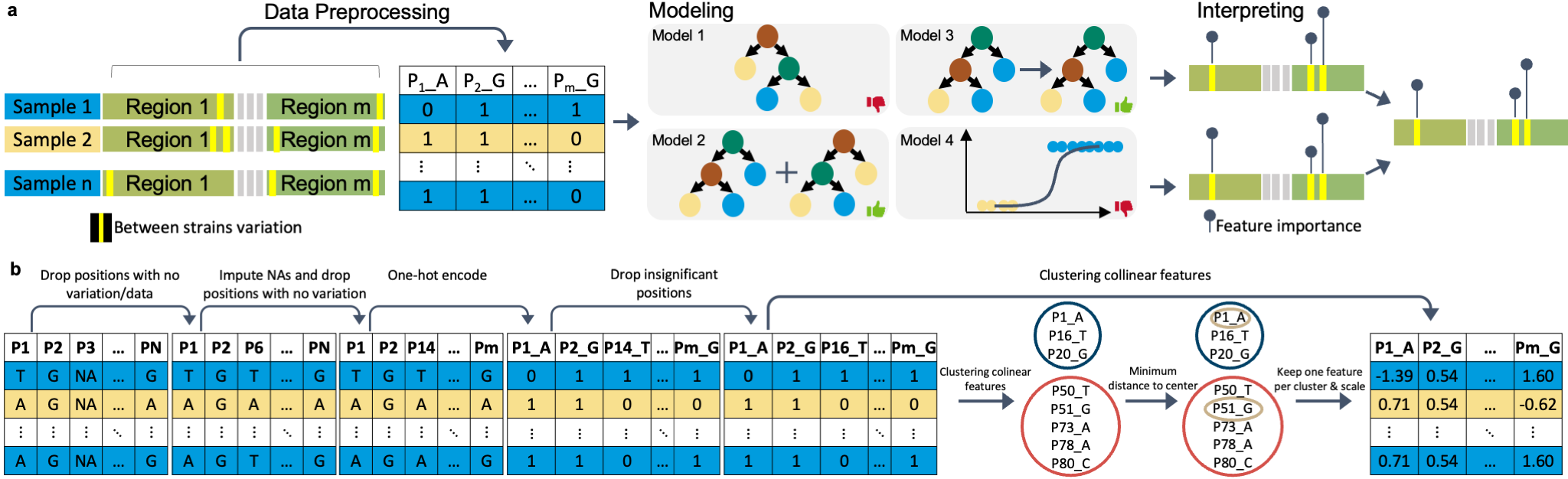
deepBreaks , a computational method, aims to identify important changes in association with the phenotype of interest using multi-alignment sequencing data from a population.
Key features:
- Generality: deepBreaks is a new computational tool for identifying genomic regions and genetic variants significantly associated with phenotypes of interest.
- Validation: A comprehensive evaluation of deepBreaks performance using synthetic data generation with known ground truth for genotype-phenotype association testing.
- Interpretation: Rather than checking all possible mutations (breaks), deepBreaks prioritizes only statistically promising candidate mutations.
- Elegance: User-friendly, open-source software allowing for high-quality visualization and statistical tests.
- Optimization: Since sequence data are often very high volume (next-generation DNA sequencing reads typically in the millions), all modules have been written and benchmarked for computing time.
- Documentation: Open-source GitHub repository of code complete with tutorials and a wide range of real-world applications.
Citation:
Mahdi Baghbanzadeh, Tyson Dawson, Bahar Sayoldin, Todd H. Oakley, Keith A. Crandall, Ali Rahnavard (2023). deepBreaks: a machine learning tool for identifying and prioritizing genotype-phenotype associations , https://github.com/omicsEye/deepBreaks/.
deepBreaks user manual
Contents
Features
- Generic software that can handle any kind of sequencing data and phenotypes
- One place to do all analysis and producing high-quality visualizations
- Optimized computation
- User-friendly software
- Provides a predictive power of most discriminative positions in a sequencing data
DeepBreaks
Installation
- First install conda
Go to the Anaconda website and download the latest version for your operating system. - For Windows users: do not forget to add
condato your systempath - Second is to check for conda availability
open a terminal (or command line for Windows users) and run:
conda --version
it should out put something like:
conda 4.9.2
if not, you must make conda available to your system for further steps. if you have problems adding conda to PATH, you can find instructions here.
Windows Linux Mac
If you are using an Apple M1/M2 MAC please go to the Apple M1/M2 MAC for installation
instructions.
If you have a working conda on your system, you can safely skip to step three.
If you are using windows, please make sure you have both git and Microsoft Visual C++ 14.0 or greater installed.
install git
Microsoft C++ build tools
In case you face issues with this step, this link may help you.
- Create a new conda environment (let's call it deepBreaks_env) with the following command:
conda create --name deepBreaks_env python=3.9
- Activate your conda environment:
conda activate deepBreaks_env
- Install deepBreaks: install with pip:
pip install deepBreaks
or you can directly install if from GitHub:
python -m pip install git+https://github.com/omicsEye/deepbreaks
Apple M1/M2 MAC
- Update/install Xcode Command Line Tools
xcode-select --install
- Install Brew
/bin/bash -c "$(curl -fsSL https://raw.githubusercontent.com/Homebrew/install/HEAD/install.sh)"
- Install libraries for brew
brew install cmake libomp
- Install miniforge
brew install miniforge
- Close the current terminal and open a new terminal
- Create a new conda environment (let's call it deepBreaks_env) with the following command:
conda create --name deepBreaks_env python=3.9
- Activate the conda environment
conda activate deepBreaks_env
- Install packages from Conda
conda install -c conda-forge lightgbm
pip install xgboost
- Finally, install deepBreaks: install with pip:
pip install deepBreaks
or you can directly install if from GitHub:
python -m pip install git+https://github.com/omicsEye/deepbreaks
Getting Started with deepBreaks
Test deepBreaks
To test if deepBreaks is installed correctly, you may run the following command in the terminal:
deepBreaks -h
Which yields deepBreaks command line options.
Options
$ deepBreaks -h
Input
usage: deepBreaks [-h] --seqfile SEQFILE --seqtype SEQTYPE --meta_data META_DATA --metavar METAVAR [--gap GAP] [--miss_gap MISS_GAP]
                  [--ult_rare ULT_RARE] --anatype {reg,cl}
                  [--distance_metric {correlation,hamming,jaccard,normalized_mutual_info_score,adjusted_mutual_info_score,adjusted_rand_score}]
                  [--fraction FRACTION] [--redundant_threshold REDUNDANT_THRESHOLD] [--distance_threshold DISTANCE_THRESHOLD]
                  [--top_models TOP_MODELS] [--cv CV] [--separate_cv] [--tune] [--plot] [--write]

options:
  -h, --help            show this help message and exit
  --seqfile SEQFILE, -sf SEQFILE
                        files contains the sequences
  --seqtype SEQTYPE, -st SEQTYPE
                        type of sequence: 'nu' for nucleotides or 'aa' for amino-acid
  --meta_data META_DATA, -md META_DATA
                        files contains the meta data
  --metavar METAVAR, -mv METAVAR
                        name of the meta var (response variable)
  --gap GAP, -gp GAP    Threshold to drop positions that have GAPs above this proportion. Default value is 0.7 and it means that the positions that
                        70% or more GAPs will be dropped from the analysis.
  --miss_gap MISS_GAP, -mgp MISS_GAP
                        Threshold to impute missing values with GAP. Gapsin positions that have missing values (gaps) above this proportionare
                        replaced with the term 'GAP'. the rest of the missing valuesare replaced by the mode of each position.
  --ult_rare ULT_RARE, -u ULT_RARE
                        Threshold to modify the ultra rare cases in each position.
  --anatype {reg,cl}, -a {reg,cl}
                        type of analysis
  --distance_metric {correlation,hamming,jaccard,normalized_mutual_info_score,adjusted_mutual_info_score,adjusted_rand_score}, -dm {correlation,hamming,jaccard,normalized_mutual_info_score,adjusted_mutual_info_score,adjusted_rand_score}
                        distance metric. Default is correlation.
  --fraction FRACTION, -fr FRACTION
                        fraction of main data to run
  --redundant_threshold REDUNDANT_THRESHOLD, -rt REDUNDANT_THRESHOLD
                        threshold for the p-value of the statistical tests to drop redundant features. Defaultvalue is 0.25
  --distance_threshold DISTANCE_THRESHOLD, -dth DISTANCE_THRESHOLD
                        threshold for the distance between positions to put them in clusters. features with distances <= than the threshold will be
                        grouped together. Default values is 0.3
  --top_models TOP_MODELS, -tm TOP_MODELS
                        number of top models to consider for merging the results. Default value is 5
  --cv CV, -cv CV       number of folds for cross validation. Default is 10. If the given number is less than 1,
                        then instead of CV, a train/test split approach will be used with --cv being the test size.

  --tune                After running the 10-fold cross validations, should the top selected models be tuned and finalize, or finalized only?
  --plot                plot all the individual positions that are statistically significant.Depending on your data, this process may produce many
                        plots.
  --write               During reading the fasta file we delete the positions that have GAPs over a certain threshold that can be changed in the
                        `gap_threshold` argumentin the `read_data` function. As this may change the whole FASTA file, you maywant to save the FASTA
                        file after this cleaning step.
Output
- correlated positions. We group all the colinear positions together.
- models summary. list of models and their performance metrics.
- plot of the feature importance of the top models in modelName_dpi.png format.
- csv files of feature importance based on top models containing, feature, importance, relative importance, group of the position (we group all the colinear positions together)
- plots and csv file of average of feature importance of top models.
- box plot (regression) or stacked bar plot (classification) for top positions of each model.
- pickle files of the plots and final models
- p-values of all the variables used in training of the final model
Demo
deepBreaks -sf PATH_TO_SEQUENCE.FASTA -st aa -md PATH_TO_META_DATA.tsv -mv
 META_VARIABLE_NAME -a reg  -dth 0.15 --plot --write
Tutorial
Multiple detailed jupyter notebook of deepBreaks implementation are available in the examples and the required data for the examples are also available in the data directory.
For the deepBreaks.models.model_compare function, these are the available models by default:
- Regression:
models = {
            'rf': RandomForestRegressor(n_jobs=-1, random_state=123),
            'Adaboost': AdaBoostRegressor(random_state=123),
            'et': ExtraTreesRegressor(n_jobs=-1, random_state=123),
            'gbc': GradientBoostingRegressor(random_state=123),
            'dt': DecisionTreeRegressor(random_state=123),
            'lr': LinearRegression(n_jobs=-1),
            'Lasso': Lasso(random_state=123),
            'LassoLars': LassoLars(random_state=123),
            'BayesianRidge': BayesianRidge(),
            'HubR': HuberRegressor(),
            'xgb': XGBRegressor(n_jobs=-1, random_state=123),
            'lgbm': LGBMRegressor(n_jobs=-1, random_state=123)
        }
- Classification:
models = {
            'rf': RandomForestClassifier(n_jobs=-1, random_state=123),
            'Adaboost': AdaBoostClassifier(random_state=123),
            'et': ExtraTreesClassifier(n_jobs=-1, random_state=123),
            'lg': LogisticRegression(n_jobs=-1, random_state=123),
            'gbc': GradientBoostingClassifier(random_state=123),
            'dt': DecisionTreeClassifier(random_state=123),
            'xgb': XGBClassifier(n_jobs=-1, random_state=123),
            'lgbm': LGBMClassifier(n_jobs=-1, random_state=123)
        }
The default metrics for evaluation are:
- Regression:
scores = {'R2': 'r2',
          'MAE': 'neg_mean_absolute_error',
          'MSE': 'neg_mean_squared_error',
          'RMSE': 'neg_root_mean_squared_error',
          'MAPE': 'neg_mean_absolute_percentage_error'
          }
- Classification:
scores = {'Accuracy': 'accuracy',
          'AUC': 'roc_auc_ovr',
          'F1': 'f1_macro',
          'Recall': 'recall_macro',
          'Precision': 'precision_macro'
          }
To get the ful list of available metrics, you can use:
from sklearn import metrics
print(metrics.SCORERS.keys())
The default search parameters for the models are:
import numpy as np
params = {
        'rf': {'rf__max_features': ["sqrt", "log2"]},
        'Adaboost': {'Adaboost__learning_rate': np.linspace(0.001, 0.1, num=2),
                     'Adaboost__n_estimators': [100, 200]},
        'gbc': {'gbc__max_depth': range(3, 6),
                'gbc__max_features': ['sqrt', 'log2'],
                'gbc__n_estimators': [200, 500, 800],
                'gbc__learning_rate': np.linspace(0.001, 0.1, num=2)},
        'et': {'et__max_depth': [4, 6, 8],
               'et__n_estimators': [500, 1000]},
        'dt': {'dt__max_depth': [4, 6, 8]},
        'Lasso': {'Lasso__alpha': np.linspace(0.01, 100, num=5)},
        'LassoLars': {'LassoLars__alpha': np.linspace(0.01, 100, num=5)}
    }
Attention: The names of models in the provided dict are the same with the names in the dict provided
for the params. If the name from the models dict does not match, the default sklearn parameters for that model
is then used. For example, model_compare_cv uses the xgboost with default hyperparameters.
To use the deepBreaks.models.model_compare_cv function with default parameters:
from deepBreaks.models import model_compare_cv
from deepBreaks.preprocessing import MisCare, ConstantCare, URareCare, CustomOneHotEncoder
from deepBreaks.preprocessing import FeatureSelection, CollinearCare
from deepBreaks.utils import get_models, get_scores, get_params, make_pipeline

ana_type = 'reg'  # assume that we are running a regression analysis
report_dir = 'PATH/TO/A/DIRECTORY' # to save the reports
prep_pipeline = make_pipeline(cache_dir=None,
    steps=[
        ('mc', MisCare(missing_threshold=0.25)),
        ('cc', ConstantCare()),
        ('ur', URareCare(threshold=0.05)),
        ('cc2', ConstantCare()),
        ('one_hot', CustomOneHotEncoder()),
        ('feature_selection', FeatureSelection(model_type=ana_type, alpha=0.25)),
        ('collinear_care', CollinearCare(dist_method='correlation', threshold=0.25))
    ])
report, top = model_compare_cv(X=tr, y=y, preprocess_pipe=prep_pipeline,
                               models_dict=get_models(ana_type=ana_type),
                               scoring=get_scores(ana_type=ana_type),
                               report_dir=report_dir,
                               cv=10, ana_type=ana_type, cache_dir=None)
To use a new set of models, params, or metrics you can define them in a dict:
import deepBreaks.models as ml
from sklearn.ensemble import RandomForestRegressor, AdaBoostRegressor
from sklearn.ensemble import ExtraTreesRegressor
from deepBreaks.models import model_compare_cv
from deepBreaks.preprocessing import MisCare, ConstantCare, URareCare, CustomOneHotEncoder
from deepBreaks.preprocessing import FeatureSelection, CollinearCare
from deepBreaks.utils import get_models, get_scores, get_params, make_pipeline

ana_type = 'reg'  # assume that we are running a regression analysis
report_dir = 'PATH/TO/A/DIRECTORY' # to save the reports
# define a new set of models
models = {'rf': RandomForestRegressor(n_jobs=-1, random_state=123),
          'Adaboost': AdaBoostRegressor(random_state=123),
          'et': ExtraTreesRegressor(n_jobs=-1, random_state=123)
          }


prep_pipeline = make_pipeline(cache_dir=None,
    steps=[
        ('mc', MisCare(missing_threshold=0.25)),
        ('cc', ConstantCare()),
        ('ur', URareCare(threshold=0.05)),
        ('cc2', ConstantCare()),
        ('one_hot', CustomOneHotEncoder()),
        ('feature_selection', FeatureSelection(model_type=ana_type, alpha=0.25)),
        ('collinear_care', CollinearCare(dist_method='correlation', threshold=0.25))
    ])
report, top = model_compare_cv(X=tr, y=y, preprocess_pipe=prep_pipeline,
                               models_dict=models,
                               scoring=get_scores(ana_type=ana_type),
                               report_dir=report_dir,
                               cv=10, ana_type=ana_type, cache_dir=None)

'''
Since we do not define a set of parameters for the model "et", it will fit with
default parameters
'''
# change the set of metrics
scores = {'R2': 'r2',
          'MAE': 'neg_mean_absolute_error',
          'MSE': 'neg_mean_squared_error'
          }

report, top = model_compare_cv(X=tr, y=y, preprocess_pipe=prep_pipeline,
                               models_dict=models,
                               scoring=scores,
                               report_dir=report_dir,
                               cv=10, ana_type=ana_type, cache_dir=None)
Applications
Here we try to use the deepBreaks on different datasets and elaborate on the results.
deepBreaks identifies amino acids associated with color sensitivity
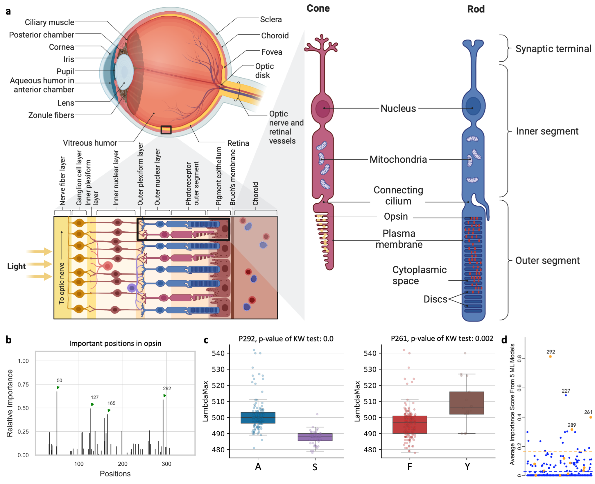
Opsins are genes involved in light sensitivity and vision, and when coupled with a light-reactive chromophore, the absorbance of the resulting photopigment dictates physiological phenotypes like color sensitivity. We analyzed the amino acid sequence of rod opsins because previously published mutagenesis work established mechanistic connections between 12 specific amino acid sites and phenotypes Yokoyama et al. (2008). Therefore, we hypothesized that machine learning approaches could predict known associations between amino acid sites and absorbance phenotypes. We identified opsins expressed in rod cells of vertebrates (mainly marine fishes) with absorption spectra measurements (λmax, the wavelength with the highest absorption). The dataset contains 175 samples of opsin sequences. We next applied deepBreaks on this dataset to find the most important sites contributing to the variations of λmax. This Jupyter Notebook illustrates the steps.
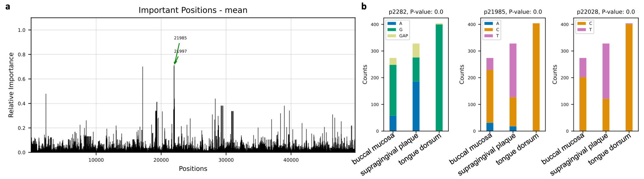
Novel insights of niche associations in the oral microbiome
Microbial species tend to adapt at the genome level to the niche in which they live. We hypothesize
that genes with essential functions change based on where microbial species live. Here we use microbial strain
representatives from stool metagenomics data of healthy adults from the
Human Microbiome Project. The input for deepBreaks consists of 1) an MSA file
with 1006 rows, each a representative strain of a specific microbial species, here Haemophilus parainfluenzae, with
49839 lengths; and 2) labels for deepBreaks prediction are body sites from which samples were collected.
This Jupyter Notebook
illustrates the steps.
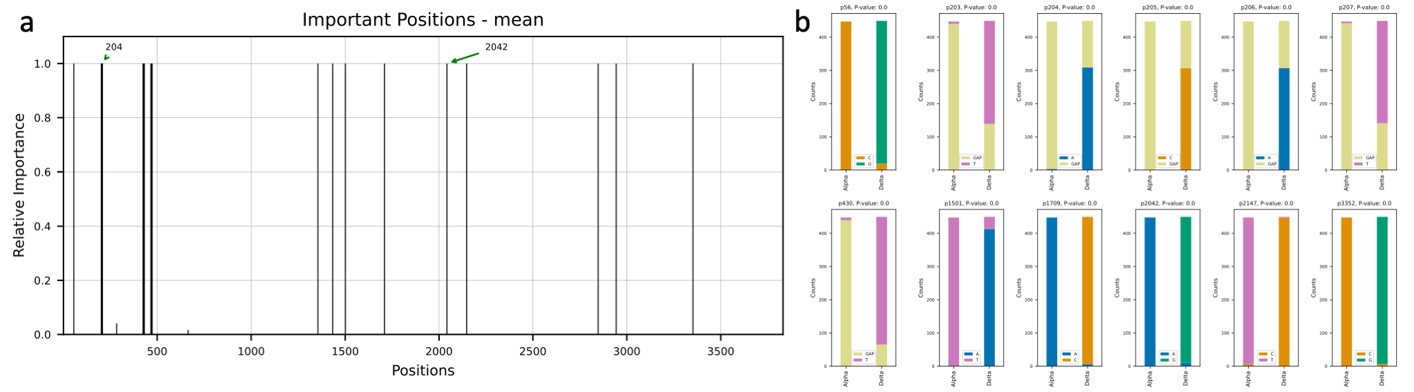
deepBreaks reveals important SARS-CoV-2 regions associated with Alpha and Delta variants
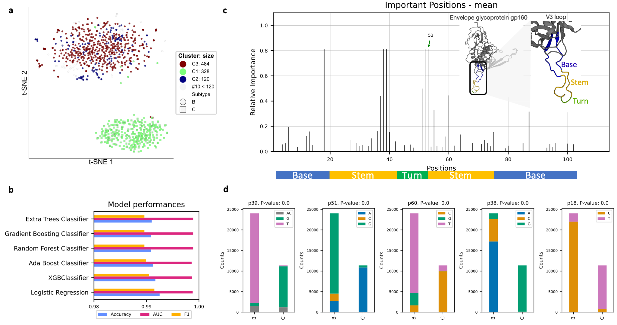
deepBreaks identifies HIV regions with potentially important functions
Support
- Please submit your questions or issues with the software at Issues tracker.
- For community discussions, questions, and issue reporting, please visit our forum here


Download files
Download the file for your platform. If you're not sure which to choose, learn more about installing packages.
Source Distribution
File details
Details for the file deepBreaks-1.1.2.tar.gz.
File metadata
- Download URL: deepBreaks-1.1.2.tar.gz
- Upload date:
- Size: 37.9 kB
- Tags: Source
- Uploaded using Trusted Publishing? No
- Uploaded via: twine/4.0.2 CPython/3.9.16
File hashes
| Algorithm | Hash digest | |
|---|---|---|
| SHA256 |
3f8c0273e82d2c0eddbd8a17358f362de41257cdeca52372c91a81e1cfea04c2
|
|
| MD5 |
b9f3b10e24e6d3a6cff250414cbf7828
|
|
| BLAKE2b-256 |
26afd10105f783ee7d848d54fb0d59025647bdec134ee24e25999b4de537a56c
|


