Dispersion-compensated algorithm for electromagnetic waveguides

Project description
Dispersion-Compensated Algorithm


Dispersion-Compensated Algorithm for the Analysis for Electromagnetic Waveguides
This package allows you to map dispersive waveguide data from the frequency-domain to distance-domain, and vice versa. The benefit of this approach, compared to a standard Fourier transform, is that this algorithm compensates for dispersion. Normally, dispersion causes signals in the time-domain to broaden as the propagate, making it difficult to isolate or supress adjacent signals. In the distance-domain, the signals remain sharp, even over long distances, allowing you to easily identify, isolate or suppress specific signals.
For more information, see:
- J. D. Garrett and C. E. Tong, "A Dispersion-Compensated Algorithm for the Analysis of Electromagnetic Waveguides", IEEE Signal Processing Letters, vol. 28, pp. 1175-1179, Jun. 2021, doi: 10.1109/LSP.2021.3086695.
Getting Started
You can install the CZT package using pip:
# to install the latest release (from PyPI)
pip install czt

# to install the latest commit (from GitHub)
git clone https://github.com/garrettj403/CZT.git
cd CZT
pip install -e .

# to install dependencies for examples
pip install -e .[examples]
Example: Simple Waveguide Section
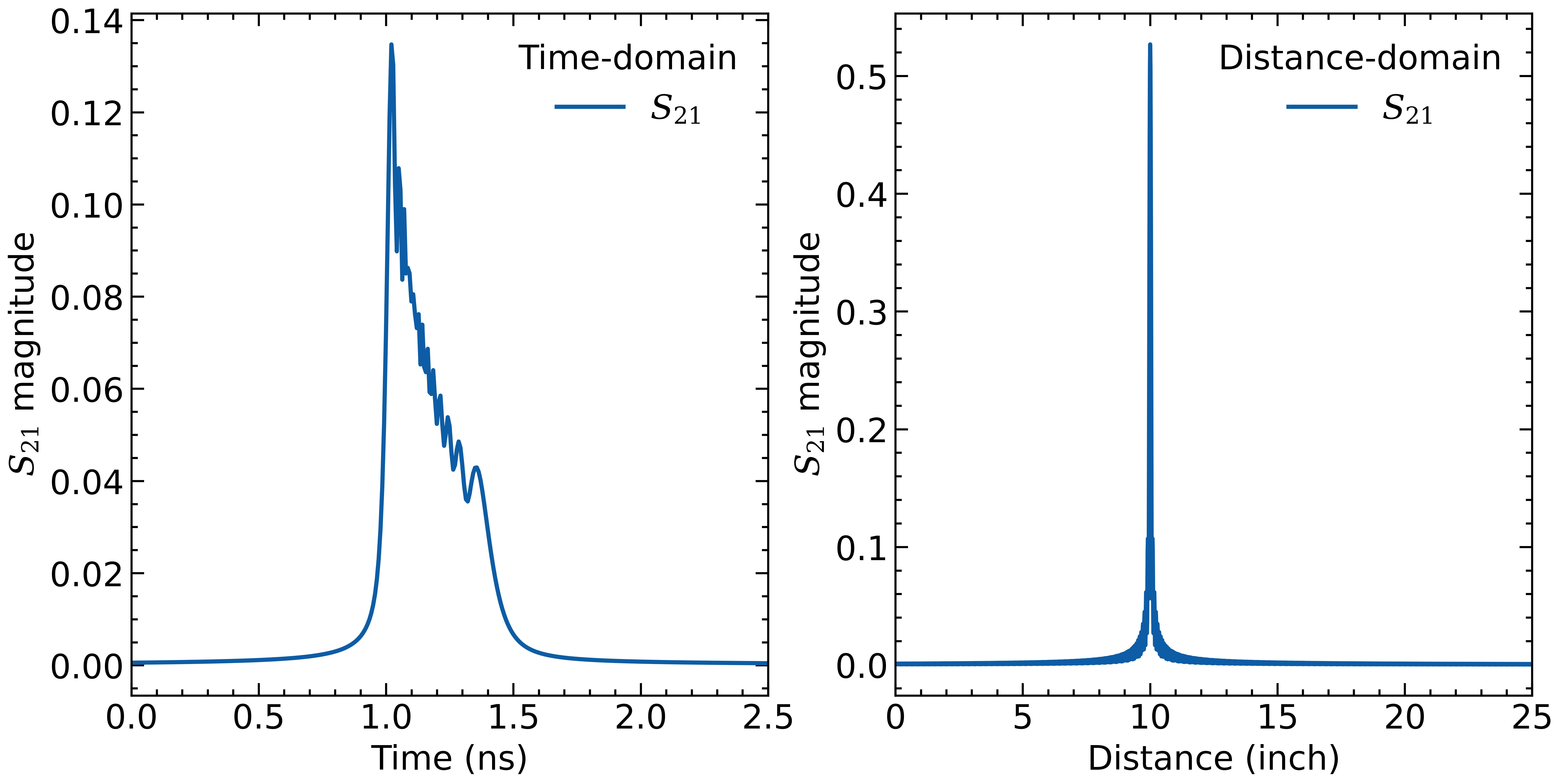
Transmission through a 10" long gold-plated WR-2.8 waveguide:
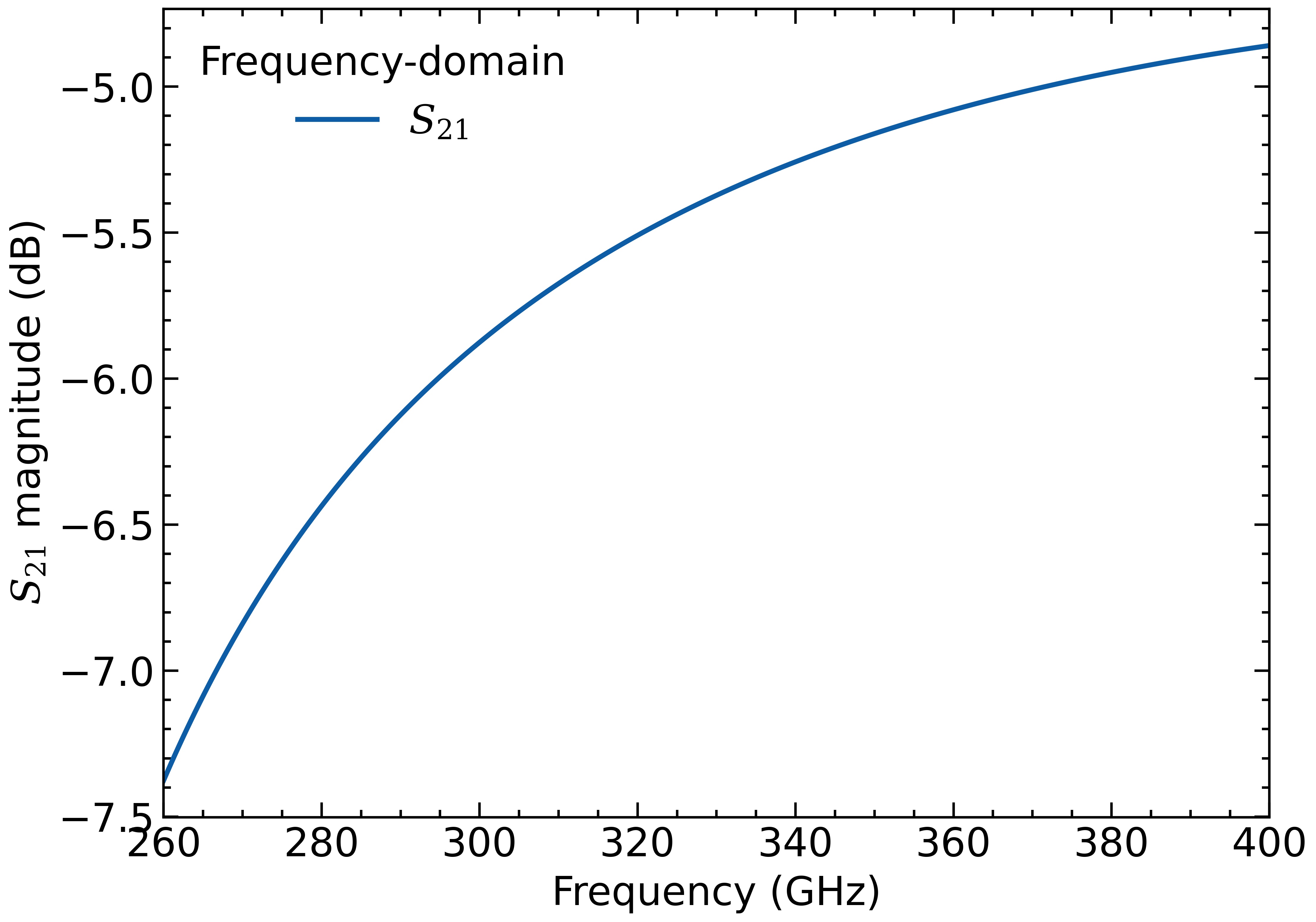
Below, the time-domain response (calculated by an IFFT) is compared to the distance-domain response. Notice how much sharper the distance-domain response is.
Example: Waveguide Cavity Resonator
This is a quick example showing the power of the dispersion-compensated algorithm. See the included notebook for more information.
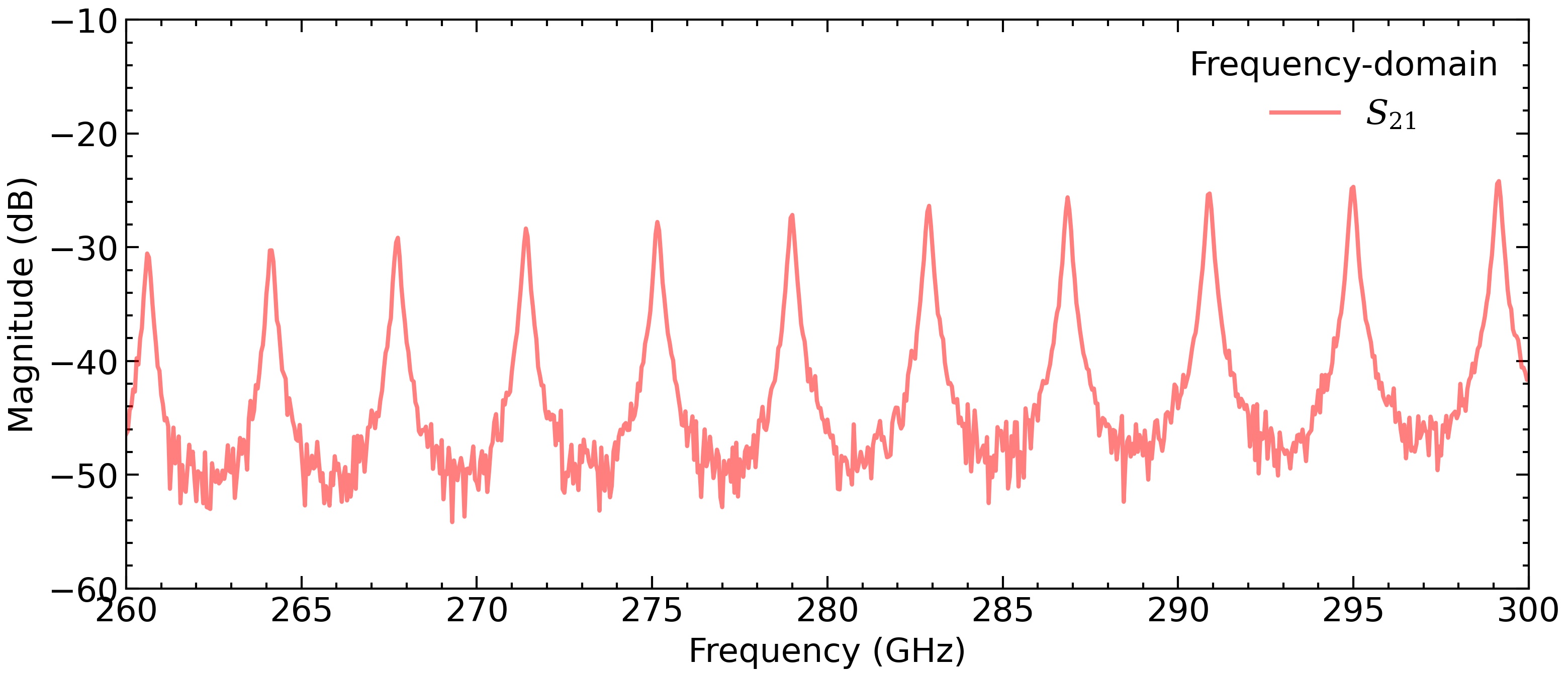
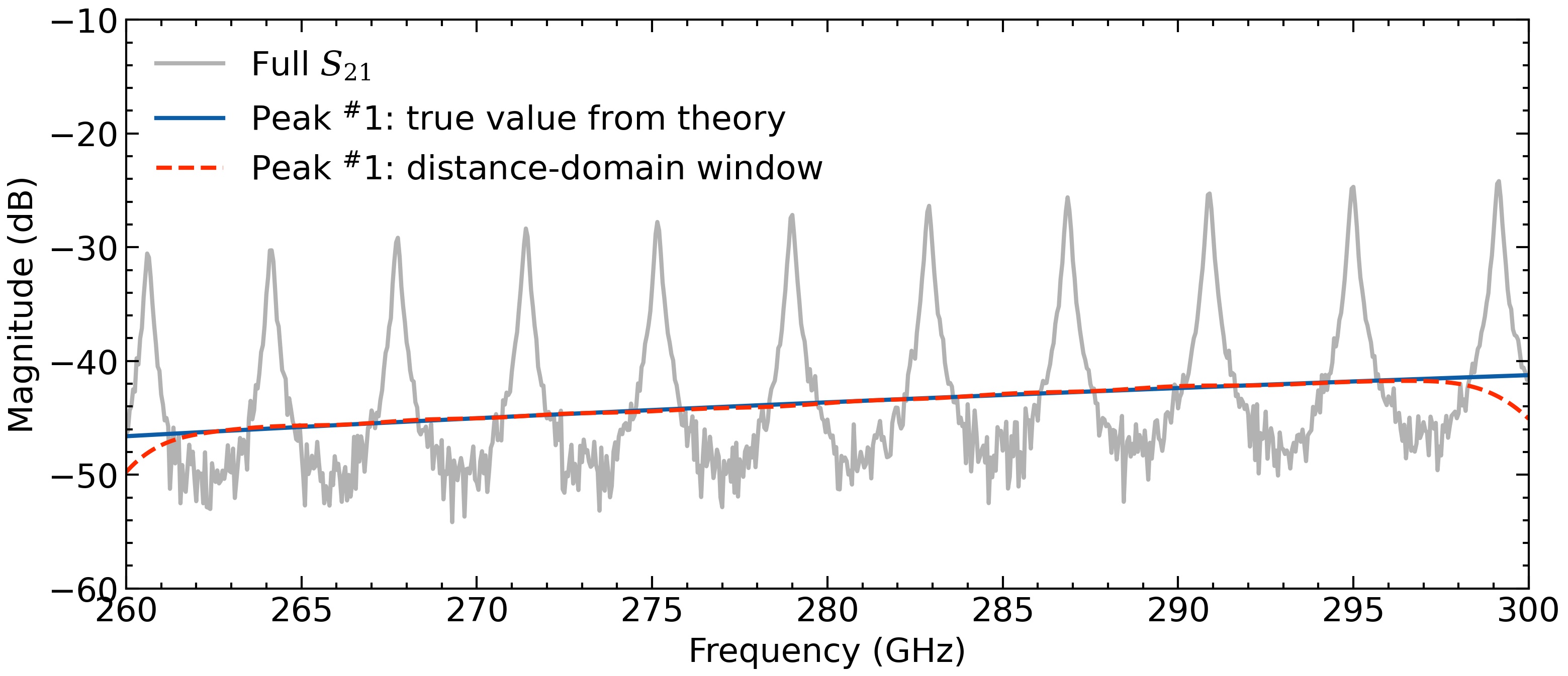
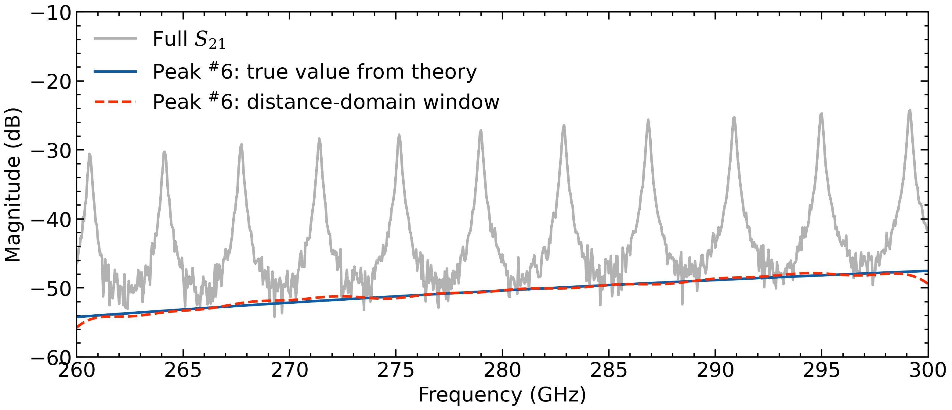
For this example, we will start with the frequency-domain response of a simple waveguide cavity resonator, as shown below. This is a 1 inch long WR-2.8 cavity. Whenever the length of the cavity is an integer number of the guided wavelength divided by two, there is a peak in transmission.
In the distance-domain, we can see a series of reflections corresponding to different signal paths within the resonator. The first peak is the signal passing straight through the resonator (distance = 1 inch), the second peak is the signal that undergoes ones internal back-and-forth reflection (distance = 3 inch), etc.
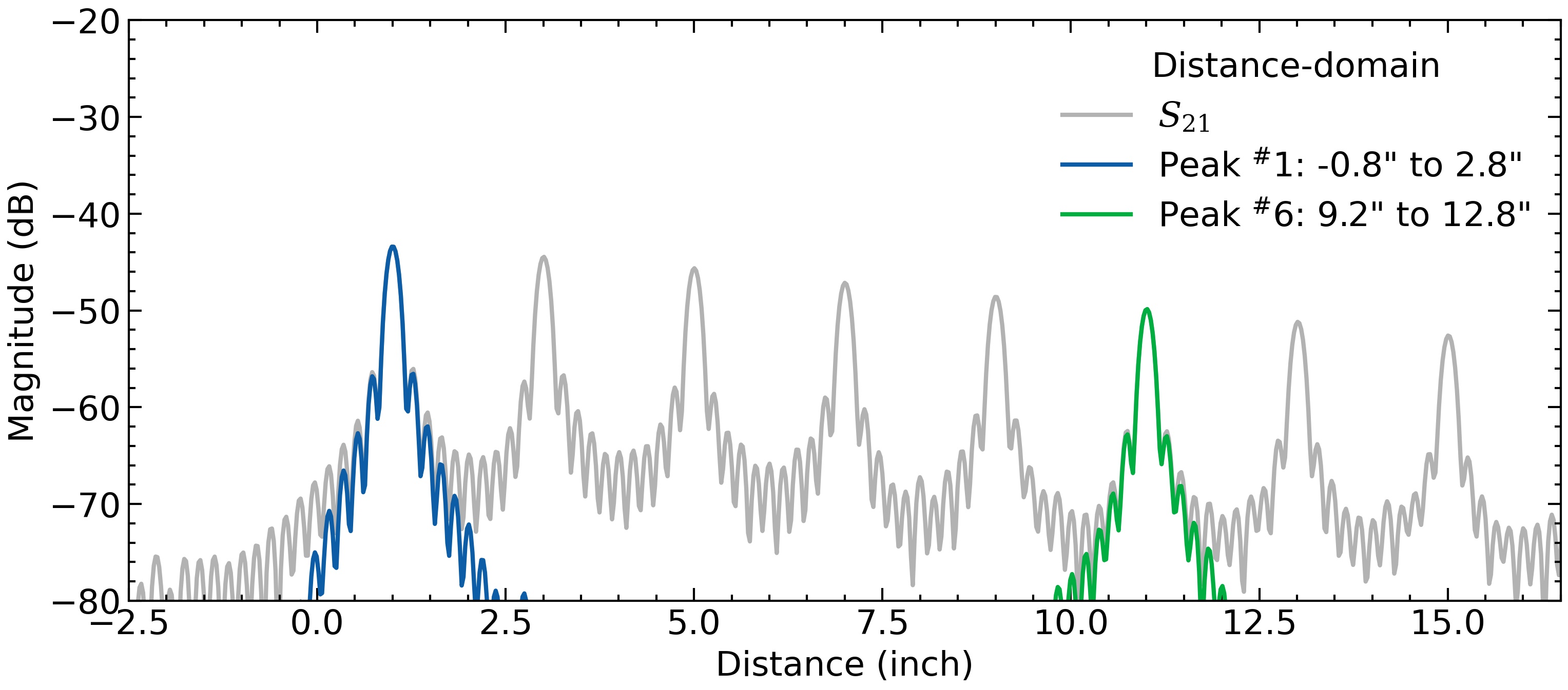
In the distance-domain, we can easily isolate the first peak and then return to the frequency-domain. The isolated reflection provides a very close match to theory.
Likewise, we can easily isolate the 6th peak and return to the frequency-domain. This is impossible in the time-domain because there is too much broadening and overlap between adjacent reflections.
Note: This example is similar to the example presented by Garrett & Tong 2021, but it is slightly different (e.g., different dimensions, different iris parameters, etc.). Please see this paper for more information.
Citing This Repo
If you use this code, please cite the following paper:
@article{Garrett2021,
  author       = {John D. Garrett and
                  Edward Tong},
  title        = {{A Dispersion-Compensated Algorithm for the Analysis of Electromagnetic Waveguides}},
  volume       = {28},
  pages        = {1175--1179},
  month        = jun,
  year         = {2021},
  journal      = {IEEE Signal Processing Letters},
  doi          = {10.1109/LSP.2021.3086695},
  url          = {https://ieeexplore.ieee.org/document/9447194}
}
Release history Release notifications | RSS feed

Download files
Download the file for your platform. If you're not sure which to choose, learn more about installing packages.
Source Distribution
File details
Details for the file disptrans-0.0.1.tar.gz.
File metadata
- Download URL: disptrans-0.0.1.tar.gz
- Upload date:
- Size: 5.1 kB
- Tags: Source
- Uploaded using Trusted Publishing? No
- Uploaded via: twine/3.4.2 importlib_metadata/3.7.3 pkginfo/1.7.1 requests/2.26.0 requests-toolbelt/0.9.1 tqdm/4.62.1 CPython/3.8.11
File hashes
| Algorithm | Hash digest | |
|---|---|---|
| SHA256 |
db1329480063d903cd10b5d2d4fab42e9f9f7efbda5cf2ca2a3e0924542f5447
|
|
| MD5 |
ef4c3f0d189c2a72d43308f63a9d0899
|
|
| BLAKE2b-256 |
ac904d3a9638626c726d2254e5914e140eb1aaa0c4deca6f8a064fee8bc1c554
|


