
fABBA: An efficient symbolic time series approximation method





Start here: Quickstart · Runnable examples · Parameter guide · Codebook export · Architecture
Native installation and releases
The installation guide explains precompiled wheels, source builds and Cython diagnostics. The release workflow requires 33 wheels across macOS Intel/Apple Silicon, Linux x86_64/ARM64 and Windows x64/ARM64. It validates every extension and NumPy ABI compatibility before assembling a complete PyPI candidate. These are release gates; local configuration alone does not certify that every remote platform has passed.
A complete numerical roundtrip
import numpy as np
from fABBA import fABBA

x = 5 + np.sin(np.linspace(0, 4 * np.pi, 200))
model = fABBA(tol=0.01, alpha=0.1, verbose=0)
symbols = model.fit_transform(x)
y = np.asarray(model.inverse_transform(symbols, start=x[0]))
print("symbols:", symbols)
print("RMSE:", np.sqrt(np.mean((x - y) ** 2)))
print("centers [length, increment]:", model.parameters.centers)
codebook = model.parameters.to_dict()  # JSON-compatible; retain symbols and start too
Symbolization is lossy. tol bounds polygonal compression error; it is not a
bound on final symbolic reconstruction RMSE. Symbol meanings belong to their
codebook. Use JABBA to encode several series with one shared codebook.
After installing this checkout, run the self-contained examples:
python example/toy_models.py        # constant, linear, periodic, step, noisy signals
python example/export_codebook.py   # JSON export and an independent decoder
python example/tolerance_sweep.py   # polygonal versus symbolic error
python example/shared_codebook.py   # train/test features with JABBA
The ABBA methods provide a fast and accurate symbolic approximation of temporal data, making them well-suited for tasks such as compression, clustering, and classification. The fABBA library is a Python-based implementation designed to efficiently apply ABBA methods. It achieves this by first approximating a time series using a polygonal chain representation and then aggregating these polygonal segments into symbolic groups.
The fABBA library supports multiple ABBA variants, including the original ABBA method and the optimized fABBA approach. Unlike ABBA, fABBA accelerates the aggregation process by sorting polygonal pieces and leveraging early termination conditions, significantly improving computational efficiency. However, this speed-up comes at the cost of slightly reduced approximation accuracy compared to ABBA. A key distinction between fABBA and the ABBA method proposed by Elsworth and Güttel [Data Mining and Knowledge Discovery, 34:1175-1200, 2020] is that fABBA eliminates the need for repeated within-cluster-sum-of-squares computations, thereby reducing its overall computational complexity. Additionally, fABBA is fully tolerance-driven, meaning that users do not need to specify the number of symbols in advance, allowing for adaptive and flexible time series symbolization.
The methods fABBA and ABBA are designed for univariate time series, and the fABBA package provides an API for implementing them. For multivariate time series or symbolizing multiple time series with a shared codebook (commonly used in classification or downstream tasks), please use JABBA and cite [3] accordingly.
🚀 Install
fABBA supports Linux, Windows, and MacOS operating system.

This checkout requires Python >= 3.9. Runtime and build dependencies are declared
in pyproject.toml. When pip builds from source, Cython and a C compiler are
required. For a compiler-free source build, set FABBA_NO_EXTENSIONS=1 before
installation; see the testing guide.
To install the current release via PIP use:
pip install fabba
Download this repository:
git clone https://github.com/nla-group/fABBA.git
It also supports conda-forge install:

To install this package via conda-forge, run the following:
conda install -c conda-forge fabba
🏁 Examples
⭐ Compress and reconstruct a time series
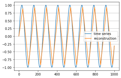
The following example approximately transforms a time series into a symbolic string representation (transform) and then converts the string back into a numerical format (inverse_transform). fABBA essentially requires two parameters tol and alpha. The tolerance tol determines how closely the polygonal chain approximation follows the original time series. The parameter alpha controls how similar time series pieces need to be in order to be represented by the same symbol. A smaller tol means that more polygonal pieces are used and the polygonal chain approximation is more accurate; but on the other hand, it will increase the length of the string representation. A smaller alpha typically results in a larger number of symbols.
The choice of parameters depends on the application, but in practice, one often just wants the polygonal chain to mimic the key features in time series and not to approximate any noise. In this example the time series is a sine wave and the chosen parameters result in the symbolic representation BbAaAaAaAaAaAaAaC. Note how the periodicity in the time series is nicely reflected in repetitions in its string representation.
import numpy as np
import matplotlib.pyplot as plt
from fABBA import fABBA

ts = [np.sin(0.05*i) for i in range(1000)]  # original time series
fabba = fABBA(tol=0.1, alpha=0.1, sorting='2-norm', scl=1, verbose=0)

string = fabba.fit_transform(ts)            # string representation of the time series
print(string)                               # prints aBbCbCbCbCbCbCbCA

inverse_ts = fabba.inverse_transform(string, ts[0]) # numerical time series reconstruction
Plot the time series and its polygonal chain reconstruction:
plt.plot(ts, label='time series')
plt.plot(inverse_ts, label='reconstruction')
plt.legend()
plt.grid(True, axis='y')
plt.show()
⭐ Load paramters
One can load the parameters via: fabba.parameters, fabba.paramters.centers.
To play fABBA further with real datasets, we recommend users start with UCI Repository and UCR Archive.
⭐ Adaptive polygonal chain approximation
Instead of using fit_transform which combines the polygonal chain approximation of the time series and the symbolic conversion into one, both steps of fABBA can be performed independently. Here’s how to obtain the compression pieces and reconstruct time series by inversely transforming the pieces:
import numpy as np
from fABBA import compress
from fABBA import inverse_compress
ts = [np.sin(0.05*i) for i in range(1000)]
pieces = compress(ts, tol=0.1)               # pieces is a list of the polygonal chain pieces
inverse_ts = inverse_compress(pieces, ts[0]) # reconstruct polygonal chain from pieces
Similarly, the digitization can be implemented after compression step as below:
from fABBA import digitize
from fABBA import inverse_digitize, quantize
string, parameters = digitize(pieces, alpha=0.1, sorting='2-norm', scl=1) # compression of the polygon
print(''.join(string))                                 # prints aBbCbCbCbCbCbCbCA

inverse_pieces = inverse_digitize(string, parameters)
inverse_ts = inverse_compress(quantize(inverse_pieces), ts[0])   # numerical time series reconstruction
⭐ Alternative ABBA approach
We also provide other clustering based ABBA methods, it is easy to use with the support of scikit-learn tools. The user guidance is as follows
import numpy as np
from sklearn.cluster import KMeans
from fABBA import ABBAbase

ts = [np.sin(0.05*i) for i in range(1000)]         # original time series
#  specifies 5 symbols using kmeans clustering
kmeans = KMeans(n_clusters=5, random_state=0, init='k-means++', n_init='auto', verbose=0)
abba = ABBAbase(tol=0.1, scl=1, clustering=kmeans)
string = abba.fit_transform(ts)                    # string representation of the time series
print(string)                                      # prints BbAaAaAaAaAaAaAaC
inverse_ts = abba.inverse_transform(string)        # reconstruction
fABBA is an extensive package, which includes all ABBA variants, you can use the original ABBA method via
from fABBA import ABBA
abba = ABBA(tol=0.1, scl=1, k=5, verbose=0)
string = abba.fit_transform(ts)
print(string)
inverse_ts = abba.inverse_transform(string, ts[0])
⭐ For multiple time series data transform
Load JABBA package and data:
from fABBA import JABBA
from fABBA import loadData
train, test = loadData()
Built in JABBA provide parameter of init for the specification of ABBA methods, if set agg, then it will automatically turn to fABBA method, and if set it to k-means, it will turn to ABBA method automatically. Use JABBA object to fit and symbolize the train set via API fit_transform, and reconstruct the time series from the symbolic representation simply by
jabba = JABBA(tol=0.0005, init='agg', verbose=1)
symbols = jabba.fit_transform(train)
reconst = jabba.inverse_transform(symbols)
Note: function loadData() is a lightweight API for time series dataset loading, which only supports part of data in UEA or UCR Archive, please refer to the document for full use detail. JABBA is used to process multiple time series as well as multivariate time series, so the input should be ensured to be 2-dimensional, for example, when loading the UCI dataset, e.g., Beef, use symbols = jabba.fit_transform(train) , when loading UEA dataset, e.g., BasicMotions, use symbols = jabba.fit_transform(train[0]) . For details, we refer to (https://www.cs.ucr.edu/~eamonn/time_series_data_2018/).
For the out-of-sample data, use the function transform to symbolize the test time series, and reconstruct the symbolization via function inverse_transform, the code illustration is as follows:
test_symbols, start_set = jabba.transform(test) # if UEA time series is used, simply use instead qabba.transform(test[0])
test_reconst = jabba.inverse_transform(test_symbols, start_set)
⭐ For symbolic approximation with quantized ABBA
Load QABBA package and data:
from fABBA import QABBA
from fABBA import loadData
train, test = loadData()
Built in QABBA provide parameter of init for the specification of ABBA methods, if set agg, then it will automatically turn to fABBA method, and if set it to k-means, it will turn to ABBA method automatically. Use QABBA object to fit and symbolize the train set via API fit_transform, and reconstruct the time series from the symbolic representation simply by
qabba = QABBA(tol=0.0005, init='agg', verbose=1, bits_for_len=8, bits_for_inc=12)
symbols = qabba.fit_transform(train)
reconst = qabba.inverse_transform(symbols)
For the out-of-sample data, use the function transform to symbolize the test time series, and reconstruct the symbolization via function inverse_transform, the code illustration is as follows:
test_symbols, start_set = qabba.transform(test) # if UEA time series is used, simply use instead jabba.transform(test[0])
test_reconst = qabba.inverse_transform(test_symbols, start_set)
⭐ For symbolic approximation with fixed point ABBA
Load XABBA package and data:
from fABBA import XABBA
from fABBA import loadData
train, test = loadData()
XABBA follows the same routine as above.
abba = XABBA(tol=0.0005, init='agg', verbose=1, bits_for_len=8, bits_for_inc=12)
symbols = abba.fit_transform(train)
reconst = abba.inverse_transform(symbols)
⭐ Image compression
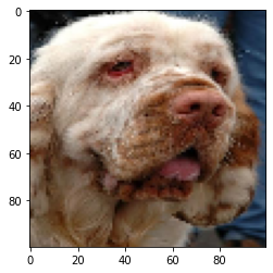
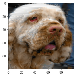
The following example shows how to apply fABBA to image data.
import matplotlib.pyplot as plt
from fABBA.load_datasets import load_images
from fABBA import image_compress
from fABBA import image_decompress
from fABBA import fABBA
from cv2 import resize
img_samples = load_images() # load test images
img = resize(img_samples[0], (100, 100)) # select the first image for test

fabba = fABBA(tol=0.1, alpha=0.01, sorting='2-norm', scl=1, verbose=1)
string = image_compress(fabba, img)
inverse_img = image_decompress(fabba, string)
Plot the original image:
plt.imshow(img)
plt.show()
Plot the reconstructed image:
plt.imshow(inverse_img)
plt.show()
🎨 Experiments
The folder "exp" contains all code required to reproduce the experiments in the manuscript "An efficient aggregation method for the symbolic representation of temporal data".
Some of the experiments also require the UCR Archive 2018 datasets which can be downloaded from UCR Time Series Classification Archive.
There are a number of dependencies listed below. Most of these modules, except perhaps the final ones, are part of any standard Python installation. We list them for completeness:
os, csv, time, pickle, numpy, warnings, matplotlib, math, collections, copy, sklearn, pandas, tqdm, tslearn
These archived experiments used NumPy >= 1.19 and < 1.20. Reproduce them in a separate historical environment; do not apply that constraint to the current package. The tested examples above use the current dependency requirements.
It is necessary to compile the Cython files in the experiments folder (though this is already compiled in the main module, the experiments code is separated). To compile the Cython extension in "src" use:
cd exp/src
python3 setup.py build_ext --inplace
or
cd exp/src
python setup.py build_ext --inplace
💌 Others
We also provide C++ implementation for fABBA in the repository cabba, it would be nice to give a shot!
Follow the build instructions in the cabba repository for the C++ implementation.
📎 Citation
If you use this repository, please kindly cite the corresponding method(s).
Thank you for supporting open research!
🔹 fABBA software (implementation / benchmarking)
Please cite:
[1] Chen, X. & Güttel, S. (2024). fABBA: A Python library for the fast symbolic approximation of time series.
Journal of Open Source Software, 9(95), 6294.
https://doi.org/10.21105/joss.06294
🔹 fABBA method (original scientific work)
Please cite:
[2] Chen, X. & Güttel, S. (2023). An efficient aggregation method for the symbolic representation of temporal data.
ACM Transactions on Knowledge Discovery from Data (TKDD), 17(1), 22.
https://doi.org/10.1145/3532622
🔹 JABBA (multivariate / multi-series symbolic approximation with shared codebook)
Please cite:
[3] Chen, X. (2024). Parallel Two-Stage Approach for Joint Symbolic Approximation of Time Series.
arXiv:2401.00109.
🔹 QABBA (quantized symbolic time series approximation)
Please cite:
[4] Carson, E., Chen, X., & Kang, C. (2025). Quantized symbolic time series approximation.
arXiv:2411.15209.
🔹 XABBA / LLM-ABBA (LLM-assisted symbolic time series representation)
Please cite:
[5] Carson, E., Chen, X., & Kang, C. (2024). LLM-ABBA: Understanding time series via symbolic approximation.
arXiv:2411.18506.
If you have any questions, please be free to reach us! You can also check our bibtex for reference.
📝 License
This project is licensed under the terms of the 
Development and validation
python -m pip install -e ".[test,docs]"
python -m unittest discover -s tests -v
python -m sphinx -W --keep-going -b html doc/source doc/_build/html
See testing and convergence contracts and local maintenance notes. The badge points to the Tests workflow; new local changes are not reflected in remote status until pushed.
1 maintainer

Metadata
1 maintainer
Release files for fABBA 1.5.3
For a detailed explanation of source distributions (sdists) and built distributions (wheels), please see the package formats documentation.
Source distribution (sdist)
| File | Size | Uploaded | |
|---|---|---|---|
| fabba-1.5.3.tar.gz | 11.7 MB | Details |
Release files / fabba-1.5.3.tar.gz
| Download URL | fabba-1.5.3.tar.gz |
|---|---|
| Size | 11.7 MB |
| Tags | Source |
|
SHA-256 checksum How to use checksums |
3a946bd31a36f354b6f10630c8fe1e079ed5ad1234ae67db14b5e34033bf6dd6
|
|
BLAKE2b-256 checksum How to use checksums |
4e140c37e874abe02049b755786ea8a0090243220d8ddcf365ad53575ea1a132
|
| Upload date | |
|
Uploaded using Trusted Publishing? What is trusted publishing? |
No |
| Uploaded via |
twine/6.1.0 CPython/3.12.11
|














