FARGO3D Wrapping

Project description
FARGOpy
Wrapping FRAGO3D


FARGOpy is a python wrapping for FARGO3D., the well-knwon hydrodynamics and magnetohydrodynamics parallel code. This wrapping is intended to ensue the interaction with FARGO3D especially for those starting using the code, for instance for teaching and training purposes, but also provide functionalities for most advanced users in tasks related to the postprocessing of output files and plotting.
Download and install FARGO3D
For using FARGOpy you first need to download and install FARGO3D and all its prerequisites. For a detailed guide please see the FARGO documentation or the project repo at bitbucket. Still, FARGOpy provides some useful commands and tools to test the platform on which you are working and check if it is prepared to use the whole functionalities of the packages or part of them.
NOTE: It is important to understand that
FARGO3Dworks especially well on Linux plaforms (includingMacOS). The same condition applies forFARGOpy. Because of that, most internal as well as public features of the packages are designed to work in aLinuxenvironment. For working in another operating systems, for instance for teaching or training purposes, please consider to use virtual machines.
Still, fargopy provides a simple way to get the latest version of FARGO3D. For this just run in the terminal:
$ ifargopy download
A copy of FARGO3D will be download in the directory where the command is executed with the name ./fargo3d/
Quickstart
There are three modalities for using fargopy:
-
FARGO3D expert. In this modality you already have a
FARGO3Dinstallation and want to usefargopyto manipulate input and output files. -
FARGO3D newbie. In this modality you are starting to use
FARGO3Dand want to use some of the tools available infargopyto compile, run and analyse the output. -
Something in the middle.
In the following we will explain the basic functionalities that might result useful in each modality.
For this quickstart let's load these utilities:
import numpy as np
import matplotlib.pyplot as plt
from IPython.display import HTML
FARGO3D expert mode
To use fargopy in the case that you already have some simulation results, run the ifargopy script:
$ ifargopy
This command will start a session of IPython and initialize fargopy. Alternatively you may prefer to work in a Jupyter notebook. In both cases, the first thing to do is to import fargopy.
import fargopy as fp
from fargopy import DEG, RAD
%load_ext autoreload
%autoreload 2
The autoreload extension is already loaded. To reload it, use:
  %reload_ext autoreload
When you run fargopy from the command line using ifargopy the previous import command is included in the initialization script.
NOTE: For the purpose of this example, we will assume that you already have a copy of
FARGO3Din a directory named./fargo3d/. Additionally we assume that for illustration purposes you have ran thefargosetup and have all or part of the outputs in the folder./fargo3d/outputs/fargo. If you have never used fargo3d, and still want to use this part of the Quickstart, ran these commands in the terminal (still, a more detailed guide toFARGO3Dand how to compile, configure and run it is described in the newbie section of this Quickstart):
ifargopy download
cd fargo3d/
make SETUP=fargo
./fargo3d setups/fargo/fargo.par
Basic commands
Any operation in fargopy requires the creation of a simulation:
sim = fp.Simulation()
Set the directory where the outputs are located:
sim.set_output_dir('./fargo3d/outputs/fargo')
Now you are connected with output directory './fargo3d/outputs/fargo'
List the files available in the output directory:
outputs = sim.list_outputs()
271 files in output directory
IDL.var, bigplanet0.dat, dims.dat, domain_x.dat, domain_y.dat, domain_z.dat, gasdens0.dat, gasdens0_2d.dat, gasdens1.dat, gasdens10.dat,
gasdens11.dat, gasdens12.dat, gasdens13.dat, gasdens14.dat, gasdens15.dat, gasdens16.dat, gasdens17.dat, gasdens18.dat, gasdens19.dat, gasdens2.dat,
gasdens20.dat, gasdens21.dat, gasdens22.dat, gasdens23.dat, gasdens24.dat, gasdens25.dat, gasdens26.dat, gasdens27.dat, gasdens28.dat, gasdens29.dat,
gasdens3.dat, gasdens30.dat, gasdens31.dat, gasdens32.dat, gasdens33.dat, gasdens34.dat, gasdens35.dat, gasdens36.dat, gasdens37.dat, gasdens38.dat,
gasdens39.dat, gasdens4.dat, gasdens40.dat, gasdens41.dat, gasdens42.dat, gasdens43.dat, gasdens44.dat, gasdens45.dat, gasdens46.dat, gasdens47.dat,
gasdens48.dat, gasdens49.dat, gasdens5.dat, gasdens50.dat, gasdens6.dat, gasdens7.dat, gasdens8.dat, gasdens9.dat, gasenergy0.dat, gasenergy1.dat,
gasenergy10.dat, gasenergy11.dat, gasenergy12.dat, gasenergy13.dat, gasenergy14.dat, gasenergy15.dat, gasenergy16.dat, gasenergy17.dat, gasenergy18.dat, gasenergy19.dat,
gasenergy2.dat, gasenergy20.dat, gasenergy21.dat, gasenergy22.dat, gasenergy23.dat, gasenergy24.dat, gasenergy25.dat, gasenergy26.dat, gasenergy27.dat, gasenergy28.dat,
gasenergy29.dat, gasenergy3.dat, gasenergy30.dat, gasenergy31.dat, gasenergy32.dat, gasenergy33.dat, gasenergy34.dat, gasenergy35.dat, gasenergy36.dat, gasenergy37.dat,
gasenergy38.dat, gasenergy39.dat, gasenergy4.dat, gasenergy40.dat, gasenergy41.dat, gasenergy42.dat, gasenergy43.dat, gasenergy44.dat, gasenergy45.dat, gasenergy46.dat,
gasenergy47.dat, gasenergy48.dat, gasenergy49.dat, gasenergy5.dat, gasenergy50.dat, gasenergy6.dat, gasenergy7.dat, gasenergy8.dat, gasenergy9.dat, gasvx0.dat,
gasvx0_2d.dat, gasvx1.dat, gasvx10.dat, gasvx11.dat, gasvx12.dat, gasvx13.dat, gasvx14.dat, gasvx15.dat, gasvx16.dat, gasvx17.dat,
gasvx18.dat, gasvx19.dat, gasvx2.dat, gasvx20.dat, gasvx21.dat, gasvx22.dat, gasvx23.dat, gasvx24.dat, gasvx25.dat, gasvx26.dat,
gasvx27.dat, gasvx28.dat, gasvx29.dat, gasvx3.dat, gasvx30.dat, gasvx31.dat, gasvx32.dat, gasvx33.dat, gasvx34.dat, gasvx35.dat,
gasvx36.dat, gasvx37.dat, gasvx38.dat, gasvx39.dat, gasvx4.dat, gasvx40.dat, gasvx41.dat, gasvx42.dat, gasvx43.dat, gasvx44.dat,
gasvx45.dat, gasvx46.dat, gasvx47.dat, gasvx48.dat, gasvx49.dat, gasvx5.dat, gasvx50.dat, gasvx6.dat, gasvx7.dat, gasvx8.dat,
gasvx9.dat, gasvy0.dat, gasvy0_2d.dat, gasvy1.dat, gasvy10.dat, gasvy11.dat, gasvy12.dat, gasvy13.dat, gasvy14.dat, gasvy15.dat,
gasvy16.dat, gasvy17.dat, gasvy18.dat, gasvy19.dat, gasvy2.dat, gasvy20.dat, gasvy21.dat, gasvy22.dat, gasvy23.dat, gasvy24.dat,
gasvy25.dat, gasvy26.dat, gasvy27.dat, gasvy28.dat, gasvy29.dat, gasvy3.dat, gasvy30.dat, gasvy31.dat, gasvy32.dat, gasvy33.dat,
gasvy34.dat, gasvy35.dat, gasvy36.dat, gasvy37.dat, gasvy38.dat, gasvy39.dat, gasvy4.dat, gasvy40.dat, gasvy41.dat, gasvy42.dat,
gasvy43.dat, gasvy44.dat, gasvy45.dat, gasvy46.dat, gasvy47.dat, gasvy48.dat, gasvy49.dat, gasvy5.dat, gasvy50.dat, gasvy6.dat,
gasvy7.dat, gasvy8.dat, gasvy9.dat, monitor, orbit0.dat, outputgas.dat, planet0.dat, summary0.dat, summary1.dat, summary10.dat,
summary11.dat, summary12.dat, summary13.dat, summary14.dat, summary15.dat, summary16.dat, summary17.dat, summary18.dat, summary19.dat, summary2.dat,
summary20.dat, summary21.dat, summary22.dat, summary23.dat, summary24.dat, summary25.dat, summary26.dat, summary27.dat, summary28.dat, summary29.dat,
summary3.dat, summary30.dat, summary31.dat, summary32.dat, summary33.dat, summary34.dat, summary35.dat, summary36.dat, summary37.dat, summary38.dat,
summary39.dat, summary4.dat, summary40.dat, summary41.dat, summary42.dat, summary43.dat, summary44.dat, summary45.dat, summary46.dat, summary47.dat,
summary48.dat, summary49.dat, summary5.dat, summary50.dat, summary6.dat, summary7.dat, summary8.dat, summary9.dat, tqwk0.dat, used_rad.dat,
variables.par,
The files describing the basic properties of the simulations are dims.dat, variables.par and domain_*.dat. You may load the information in these files:
vars, domains = sim.load_properties()
Loading variables
84 variables loaded
Simulation in 2 dimensions
Loading domain in cylindrical coordinates:
	Variable phi: 384 [[0, -3.1334114227210694], [-1, 3.1334114227210694]]
	Variable r: 128 [[0, 0.408203125], [-1, 2.491796875]]
	Variable z: 1 [[0, 0.0], [-1, 0.0]]
Configuration variables and domains load into the object. See e.g. <sim>.vars
Load field data into memory
The outputs of a simulation are given as datafiles containing the value of different fields in the coordinate grid. You can load a single field:
gasdens0 = sim.load_field('gasdens',snapshot=0)
gasdens0, gasdens0.data.shape
([[[0.00063662 0.00063662 0.00063662 ... 0.00063662 0.00063662 0.00063662]
   [0.00063662 0.00063662 0.00063662 ... 0.00063662 0.00063662 0.00063662]
   [0.00063662 0.00063662 0.00063662 ... 0.00063662 0.00063662 0.00063662]
   ...
   [0.00063662 0.00063662 0.00063662 ... 0.00063662 0.00063662 0.00063662]
   [0.00063662 0.00063662 0.00063662 ... 0.00063662 0.00063662 0.00063662]
   [0.00063662 0.00063662 0.00063662 ... 0.00063662 0.00063662 0.00063662]]],
 (1, 128, 384))
As you can see, fields are loaded as special Field objects (see fp.Field? for a list of attributes and methods), whose most important attribute is data which is the numpy array containing the values of the field in the coordinate domain.
Vectorial fields are special cases. In FARGO3D each component of the field is separated by file suffixes such as x, y and z (even if you are working in different coordinate systems). fargopy is able to load all components if a vector field using:
vel = sim.load_field('gasv',snapshot=0,type='vector')
vel.data.shape
(2, 1, 128, 384)
As you can see, the first index correspond to the component of the field (x and y in the FARGO3D convention, but actually phi and r in cylindrical coordinates). The second index is the z coordinate, the third the y coordinate (r in the cylindrical system of coordinates) and the fourh is the z coordinate (phi in the cylindrical system of coordinates).
Depending on the size of the outputs, you can also load all physical fields in the output associated to a given fluid. Use this method with caution:
fields0 = sim.load_allfields('gas',snapshot=0)
fields0.keys(), fields0.size
(['gasdens', 'gasenergy', 'gasvx', 'gasvy', 'size'], 1.5)
Size here is given in Megabytes.
If you want all the fields drop the snapshot option (or set in None):
fields = sim.load_allfields('gas')
fields.print_keys()
fields.item('0').keys(), fields.size
0, 1, 10, 11, 12, 13, 14, 15, 16, 17,
18, 19, 2, 20, 21, 22, 23, 24, 25, 26,
27, 28, 29, 3, 30, 31, 32, 33, 34, 35,
36, 37, 38, 39, 4, 40, 41, 42, 43, 44,
45, 46, 47, 48, 49, 5, 50, 6, 7, 8,
9, snapshots, size


(['gasdens', 'gasenergy', 'gasvx', 'gasvy'], 76.5)
fields.item('0').gasdens.data.shape
(1, 128, 384)
As you may see, the size of the fields start to be considerable large (36 MB in this case), so it is important to not abusing of this command.
Field slices
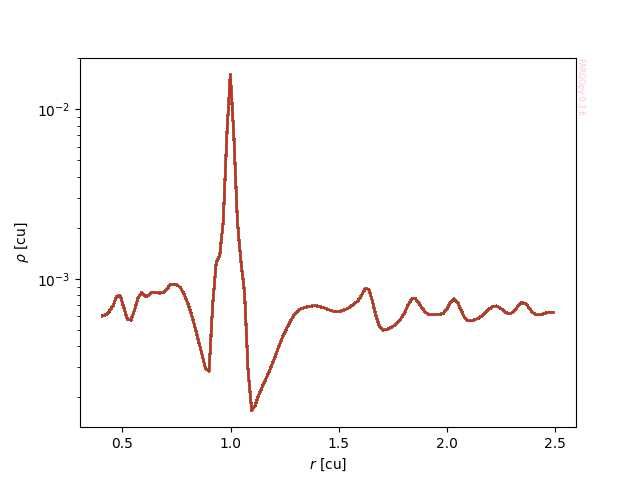
Once you have loaded a given field you may want to extract a slice for plotting. Let's for instance plot the density as a function of distance in the example simulation at a given snapshot:
gasdens10 = sim.load_field('gasdens',snapshot=10)
gasdens10.data.shape
(1, 128, 384)
Let's extract the density of the gas at phi=0 and z=0:
gasdens_r = gasdens10.slice(phi=0,z=0)
gasdens_r.shape
(128,)
And plot:
plt.ioff()
fig,ax = plt.subplots()
ax.semilogy(sim.domains.r,gasdens_r)
ax.set_xlabel(r"$r$ [cu]")
ax.set_ylabel(r"$\rho$ [cu]")
fp.Util.fargopy_mark(ax);
fig.savefig('gallery/example-dens_r.png')
We can do this in a single step with fargopy:
gasdens, mesh = gasdens10.meshslice(slice='z=0,phi=0')
The object mesh now contains matrices of the coordinates:
mesh.keys()
['r', 'phi', 'x', 'y', 'z']
If you are plotting r vs. gasdens the plot will be:
plt.ioff()
fig,ax = plt.subplots()
ax.semilogy(mesh.r,gasdens)
ax.set_xlabel(r"$r$ [cu]")
ax.set_ylabel(r"$\rho$ [cu]")
fp.Util.fargopy_mark(ax)
fig.savefig('gallery/example-dens_r.png')
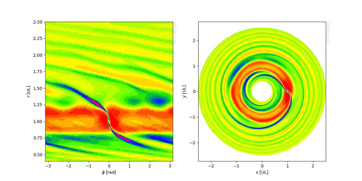
This simple procedure reduce considerably the creation of more complex plots, for instance, a map of the density in different planes:
gasdens, mesh = gasdens10.meshslice(slice='z=0')
And plot it:
plt.ioff()
fig,axs = plt.subplots(1,2,figsize=(12,6))

ax = axs[0]
ax.pcolormesh(mesh.phi*RAD,mesh.r*sim.UL/fp.AU,gasdens,cmap='prism')
ax.set_xlabel('$\phi$ [deg]')
ax.set_ylabel('$r$ [au]')
fp.Util.fargopy_mark(ax)

ax = axs[1]
ax.pcolormesh(mesh.x*sim.UL/fp.AU,mesh.y*sim.UL/fp.AU,
              gasdens,cmap='prism')
ax.set_xlabel('$x$ [au]')
ax.set_ylabel('$y$ [au]')
fp.Util.fargopy_mark(ax)
ax.axis('equal')
fig.savefig('gallery/example-dens_disk.png')
Let's create an animation for illustrating how easy FARGOpy make life:
plt.ioff()
from celluloid import Camera
from tqdm import tqdm

sim = fp.Simulation()
sim.set_output_dir('./fargo3d/outputs/fargo')
sim.load_properties()

gasdens_all = sim.load_allfields('gasdens')
fig,axs = plt.subplots(1,2,figsize=(12,6))

cmap = 'prism'
camera = Camera(fig)
for snapshot in tqdm(gasdens_all.snapshots):
    gasdens_snap = gasdens_all.item(str(snapshot)).gasdens
    gasdens,mesh = gasdens_snap.meshslice(slice='z=0')

    ax = axs[0]
    ax.pcolormesh(mesh.phi*RAD,mesh.r*sim.UL/fp.AU,gasdens,cmap=cmap)
    ax.set_xlabel('$\phi$ [deg]')
    ax.set_ylabel('$r$ [au]')

    ax = axs[1]
    ax.pcolormesh(mesh.x*sim.UL/fp.AU,mesh.y*sim.UL/fp.AU,gasdens,cmap=cmap)
    ax.set_xlabel('$x$ [au]')
    ax.set_ylabel('$y$ [au]')
    fp.Util.fargopy_mark(ax)

    camera.snap()

animation = camera.animate()
animation.save('gallery/fargo-animation.gif')
Now you are connected with output directory './fargo3d/outputs/fargo'
Loading variables
84 variables loaded
Simulation in 2 dimensions
Loading domain in cylindrical coordinates:
	Variable phi: 384 [[0, -3.1334114227210694], [-1, 3.1334114227210694]]
	Variable r: 128 [[0, 0.408203125], [-1, 2.491796875]]
	Variable z: 1 [[0, 0.0], [-1, 0.0]]
Configuration variables and domains load into the object. See e.g. <sim>.vars


100%|██████████| 51/51 [00:01<00:00, 38.16it/s]
FARGO3D newbie
This section is under development.
What's new
Version 0.2.*:
- First real applications tested with FARGOpy.
- All basic routines for reading output created.
- Major refactoring.
Version 0.1.*:
- Package is now provided with a script 'ifargopy' to run 'ipython' with fargopy initialized.
- A new 'progress' mode has been added to status method.
- All the dynamics of loading/compiling/running/stoppìng/resuming FARGO3D has been developed.
Version 0.0.*:
- First classes created.
- The project is started!
This package has been designed and written mostly by Jorge I. Zuluaga with advising and contributions by Matías Montesinos (C) 2023
Release history Release notifications | RSS feed


Download files
Download the file for your platform. If you're not sure which to choose, learn more about installing packages.
Source Distribution
Built Distribution
Filter files by name, interpreter, ABI, and platform.
If you're not sure about the file name format, learn more about wheel file names.
Copy a direct link to the current filters
File details
Details for the file fargopy-0.2.1.tar.gz.
File metadata
- Download URL: fargopy-0.2.1.tar.gz
- Upload date:
- Size: 28.1 kB
- Tags: Source
- Uploaded using Trusted Publishing? No
- Uploaded via: twine/4.0.2 CPython/3.9.16
File hashes
| Algorithm | Hash digest | |
|---|---|---|
| SHA256 |
45c9192c7815a3c78789831e8a62f92eb4c613ae9e69a792a781cf02c109cd3a
|
|
| MD5 |
3d66d8e48cf6dd7e0b055d65db332547
|
|
| BLAKE2b-256 |
aeef882ae8e69e61d23c86ff65904735be5e9668ecc9db95d4e8b7d7af192546
|
File details
Details for the file fargopy-0.2.1-py3-none-any.whl.
File metadata
- Download URL: fargopy-0.2.1-py3-none-any.whl
- Upload date:
- Size: 25.3 kB
- Tags: Python 3
- Uploaded using Trusted Publishing? No
- Uploaded via: twine/4.0.2 CPython/3.9.16
File hashes
| Algorithm | Hash digest | |
|---|---|---|
| SHA256 |
7b15f6fc7efcc2402baf43de028de0dda3b1ae7328935570cc94f7f994f89184
|
|
| MD5 |
80316b70427894dc7f520ffdfb8df9a9
|
|
| BLAKE2b-256 |
cb2276efa807441a655c614eeed609ab50532f044f90348fe7fbc0f8c1d23c6a
|


