Formability analysis in materials science.

Project description

formable provides tools for formability analysis in materials science.
Installation
pip install formable
To support showing visualisations within a Jupyter notebook, you will also need to make sure Plotly is set up to work within the notebook environment:
pip install "notebook>=5.3" "ipywidgets>=7.2"
Getting Started
LoadResponse and LoadResponseSet
The response of a material to a load is represented by the LoadResponse class. Use the following code snippet create a LoadResponse, where the arguments passed represent incremental data (i.e. data for each of the "steps" in the loading):
from formable import LoadResponse

load_response = LoadResponse(true_stress=true_stress, equivalent_strain=equivalent_strain)
true_stress and equivalent_strain are Numpy arrays of shapes (N, 3, 3) and (N,), respectively, for N increments within the load response.
A collection of load responses that contain the same incremental data are represented by the LoadResponseSet class:
from formable import LoadResponse, LoadResponseSet

all_responses = [LoadResponse(...), LoadResponse(...), ...]
load_set = LoadResponseSet(all_responses)
Yield functions
A number of yield functions as defined in the literature can be fitted and visualised. As an example, let's visualise the difference between the Von Mises and the Tresca yield criteria:
from formable.yielding.yield_functions import YieldFunction, VonMises, Tresca
von_mises = VonMises(equivalent_stress=70e6)
tresca = Tresca(equivalent_stress=70e6)
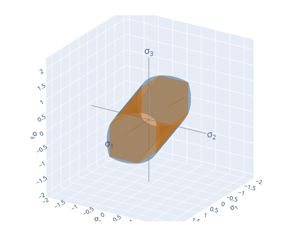
YieldFunction.compare_3D([von_mises, tresca])
If run within a Jupyter environment, this code snippet will generated a 3D visualisation of the yield surfaces in principal stress space:
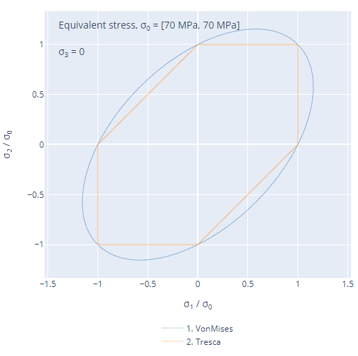
To look at a single plane within principal stress space, we can do this:
YieldFunction.compare_2D([von_mises, tresca], plane=[0, 0, 1])
which generates a figure like this:
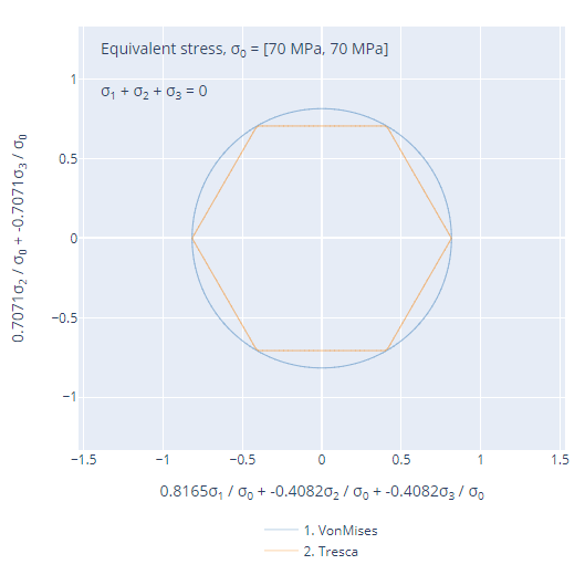
We can choose any plane that intercepts the origin. For instance, we can also look at the π-plane (σ1 = σ2 = σ3):
YieldFunction.compare_2D([von_mises, tresca], plane=[1, 1, 1])
which generates a figure like this:
Yield function fitting
Using experimental or simulated yielding tests, we can fit yield functions to the results. Consider a LoadResponseSet object that has a sufficiently large number of increments of true_stress and equivalent_strain data to enable such a fit. Using the Barlat "Yld2000-2D" anisotropic yield function as an example, we can perform a fit:
from formable import LoadResponse, LoadResponseSet
from formable.yielding import YieldPointCriteria

# First generate a LoadResponseSet, using the results from experiment/simulation:
all_responses = [LoadResponse(...), LoadResponse(...), ...]
load_set = LoadResponseSet(all_responses)

# Then define a yield point criterion:
yield_point = YieldPointCriteria('equivalent_strain', 1e-3)

# Now calculate yield stresses according to the yield point criteria:
load_set.calculate_yield_stresses(yield_point)

# Now we can fit to the resulting yield stresses:
load_set.fit_yield_function('Barlat_Yld2000_2D', equivalent_stress=70e6)
Choosing the fitting parameters and initial guesses
We can specify which of the yield function parameters we would like to fit, and which should remain fixed. We can also pass initial values to the fitting procedure. A least squares fit is employed to fit yield functions in formable.
To fix a parameter during the fit, just pass it as a keyword argument to the fit_yield_function method, as we did in the above example, where we fixed the equivalent_stress parameter. To pass initial values for some of the parameters, we can pass a initial_params dictionary:
load_set.fit_yield_function('Barlat_Yld2000_2D', initial_params={'a1': 1.4})
We can see the available parameters of a given yield function by using the PARAMETERS attribute of a YieldFunction class:
from formable.yielding.yield_functions import Barlat_Yld2000_2D

print(Barlat_Yld2000_2D.PARAMETERS)
which prints:
['a1',
 'a2',
 'a3',
 'a4',
 'a5',
 'a6',
 'a7',
 'a8',
 'equivalent_stress',
 'exponent']
Alternatively, if we have created a yield function object (from a fitting procedure, or directly), we can use the get_parameters method to get the parameters and their values:
print(von_mises.get_parameters())
which prints:
{'equivalent_stress': 70000000.0}
Visualising the fit
Once a yield function has been fit to a load set, we can visualise the fitted yield function like this:
load_set.show_yield_functions_3D()
or, in a similar way to above, we can visualise the fitted yield functions in a given principal stress plane, using:
load_set.show_yield_functions_2D(plane=[0, 0, 1])
Change Log
[0.1.21] - 2023.11.09
Fixed
- Resolve numpy deprecation.
[0.1.20] - 2022.08.08
Changed
- Constrain LM fitting process
- Relabel attribute
true_stresstostressinLoadResponseclass
[0.1.19] - 2021.11.09
Added
- Add
cyclic_uniaxialload case method to taskgenerate_load_case - Add
mixedload case method to taskgenerate_load_case
[0.1.18] - 2021.08.06
Added
- Add option
include_yield_functionstoLoadResponseSet.show_yield_functions_2DandLoadResponseSet.show_yield_functions_3D, which is a list of fitted yield function indices to include in the visualisation. - Add
get_load_case_planar_2Dload case function. - Add option
strain_rate_modetoget_load_case_plane_strain, which determines if the load case is defined by deformation gradient (F_rate), velocity gradient (L) or an approximation excluding the stress condition (L_approx), which is useful when we want to avoid using mixed boundary conditions.
Changed
- Functions
get_load_case_uniaxial,get_load_case_biaxialandget_load_case_plane_strainhave been refactored, documented and generalised where applicable. The returneddictfrom these functions now includes passing throughdirectionandrotation. A new keyrotation_matrixis the matrix representation of the rotation specified, if specified.
[0.1.17] - 2021.05.11
Added
- Add animation widget for yield func evolution:
animate_yield_function_evolution(load_response_sets, ...). - Ability to add sheet direction labels in yield function plots.
[0.1.16] - 2021.04.23
Changed
- 2D yield function plotting now use scikit-image to compute the zero-contour, which can then be plotted as scatter-plot data, instead of a Plotly contour plot. Partial fix (2D only) for #9. The old behaviour can be switched on with
use_plotly_contour=Truein methods:YieldFunction.compare_2D,YieldFunction.show_2DandLoadResponseSet.show_yield_functions_2D. - The
YieldFunction.yield_pointattribute is saved in the dict representation of a eachLoadResponseSet.fitted_yield_function, and loaded correctly when loading from a dict, via a change toYieldFunction.from_name. - Parameter fitting using the
LMFitterclass now scales the fitting parameters to one.
[0.1.15] - 2021.04.10
Fixed
- Bug fix in
LoadResponseSet.to_dictif an associated yield function was not fitted.
[0.1.14] - 2021.04.10
Added
- Add ability to specify fitting bounds and other optimisation parameters in
YieldFunction.from_fitandLoadResponseSet.fit_yield_function.
Changed
LoadResponseSet.yield_functionsattribute renamedLoadResponseSet.fitted_yield_functions.
[0.1.13] - 2021.03.28
Changed
- Do not modify input dict to
levenberg_marquardt.LMFitter.from_dict. - Fix bug in
TensileTest.show()stress scale.
Added
- Add
to_dictandfrom_dictmethods toLoadResponseSet.
[0.1.12] - 2020.12.16
Added
- Add
LMFitter.from_dict
Fixed
- Add
single_crystal_parametersto returned dict ofLMFitter.to_dict.
[0.1.11] - 2020.12.16
Fixed
- Set float values in
get_new_single_crystal_params.
[0.1.10] - 2020.12.15
Added
- Add new module,
levenberg_marquardtfor fitting single crystal parameters.
[0.1.9] - 2020.11.18
Fixed
- Add missing import to
formable.utils.
[0.1.8] - 2020.11.18
Added
- Include
tensile_testmodule fromtensile_testpackage.
[0.1.7] - 2020.09.17
Fixed
- Fix plot line colouring for many traces (more than Plotly default colour list)
[0.1.6] - 2020.08.22
Changed
- Add
dump_frequencyto load case generators.
[0.1.5] - 2020.08.18
Changed
- Default tolerance for
LoadResponse.is_uniaxialcheck loosened to 0.3.
[0.1.4] - 2020.07.01
Changed
- Print out the degree to which the stress state is uniaxial in
LoadResponse.is_uniaxial.
[0.1.3] - 2020.06.09
Added
- Add a method to estimate the Lankford coefficient via the tangent of the yield surface at a uniaxial stress state:
YieldFunction.get_numerical_lankford - Add options to
YieldFunction.show_2D,YieldFunction.compare_2DandLoadResponseSet.show_yield_functions_2Dto visualise the tangent and normal to the yield function at a uniaxial stress state. - Add incremental data:
equivalent_plastic_strainandaccumulated_shear_strain, and associatedYieldPointCriteriamappings for getting the yield stress (using the same method as that used forequivalent_stress[total]). - Add
show_stress_statestoLoadResponseSet.show_yield_functions_3DandLoadResponseset.show_yield_functions_2Dto optionally hide stress states. - Add option to pass Plotly
layoutparameters to yield function visualisation methods. - Add property
num_incrementstoLoadResponse. - Add
reprtoLoadResponseandLoadResponseSet. - Add
YieldFunction.from_name()class method for generating a yield function from a string name and parameters. - Add
LoadResponse.incremental_dataproperty to return all incremental data as adict.
Changed
- Check each
incremental_dataarray passed toLoadResponsehas the same outer shape (i.e. same number of increments). AVAILABLE_YIELD_FUNCTIONSandYIELD_FUNCTION_MAPhave been replaced with functionsget_available_yield_functionsandget_yield_function_map, respectively.- Number of excluded load responses is printed when performing yield function fitting.
[0.1.2] - 2020.05.09
Fixed
- Fixed an issue when visualising yield surfaces in 3D (via
YieldSurface.compare_3D()) (and also 2D) where, if the value of the yield function residual was already normalised (e.g. by the equivalent stress), then the isosurface drawn by Plotly was defective (showing spikes beyond the bounds of the contour grid), since the values that were being contoured were of the order 10^-8. This was because we normalised by the equivalent stress again when calculating the contour values. This was fixed by normalising by the absolute maximum value in the values that are returned by the residual function, rather than always normalising by the equivalent stress, so the contour values should be of the order 1 now, regardless of whether a given yield function residual value is normalised or not. - Fixed yield function residual for
Barlat_Yld91, where hydrostatic stresses would returnnp.nan. - Check for bad
kwargsinLoadResponseSet.fit_yield_function. - Added an
equivalent_stressparameter toHill1948to make it fit and visualise like the others. Not sure if this is the correct approach.
Added
- Added an option to show the bounds of the 3D contour grid when visualising yield functions in 3D.
- Added an option to associate additional text in visualising yield functions (for the legend):
legend_text. - Added module
load_casesfor generating load cases for simulations. - Added hover text in
YieldFunction.compare_2Dthat shows the value(s) of the yield function at each grid point. - Added
lankfordproperty toHill1948that returns the Lankford coefficient, as determined by the values of the anisotropic parameters.
Changed
- The tolerance for checking if a
uniaxial_responsepassed toLoadResponseSet.fit_yield_functionis in fact uniaxial has been loosened, since this way failing when it shouldn't have. - Normalise all yield function residuals by their equivalent stress parameter.
[0.1.1] - 2020.04.12
Changed
Image URLs in README
[0.1.0] - 2020.04.12
Initial release.
Release history Release notifications | RSS feed


Download files
Download the file for your platform. If you're not sure which to choose, learn more about installing packages.
Source Distribution
Built Distribution
Filter files by name, interpreter, ABI, and platform.
If you're not sure about the file name format, learn more about wheel file names.
Copy a direct link to the current filters
File details
Details for the file formable-0.1.21.tar.gz.
File metadata
- Download URL: formable-0.1.21.tar.gz
- Upload date:
- Size: 2.8 MB
- Tags: Source
- Uploaded using Trusted Publishing? No
- Uploaded via: twine/3.1.1 pkginfo/1.5.0.1 requests/2.28.2 setuptools/46.3.1.post20200515 requests-toolbelt/0.9.1 tqdm/4.64.1 CPython/3.8.2
File hashes
| Algorithm | Hash digest | |
|---|---|---|
| SHA256 |
092efa05f2154635ab4e95a6f300b2a62abb1c9926eebc3f4e165afc76734cd5
|
|
| MD5 |
2025f759ae9c9b31b31503bc65c0050f
|
|
| BLAKE2b-256 |
90462ae7d1d185f9645bc03e8dda1009bc7d89dbb22ebd4b2810a16defe4813a
|
File details
Details for the file formable-0.1.21-py3-none-any.whl.
File metadata
- Download URL: formable-0.1.21-py3-none-any.whl
- Upload date:
- Size: 54.1 kB
- Tags: Python 3
- Uploaded using Trusted Publishing? No
- Uploaded via: twine/3.1.1 pkginfo/1.5.0.1 requests/2.28.2 setuptools/46.3.1.post20200515 requests-toolbelt/0.9.1 tqdm/4.64.1 CPython/3.8.2
File hashes
| Algorithm | Hash digest | |
|---|---|---|
| SHA256 |
b0b8fbeb84b6889f1b43da87461dd3b3a4dab5cf24f4c6203e10524384918bb1
|
|
| MD5 |
2bc2034f80f46aebdae9f93ac122474f
|
|
| BLAKE2b-256 |
dfd10429c87ef77ddfa735a8e27393006df543877fea2fc59dcbb74197c5542d
|


