A fast minimum-weight perfect matching solver for quantum error correction

Project description


Fusion Blossom
A fast Minimum-Weight Perfect Matching (MWPM) solver for Quantum Error Correction (QEC)
Key Features
- Linear Complexity: The decoding time is roughly $O(N)$, proportional to the number of syndrome vertices $N$.
- Parallelism: A single MWPM decoding problem can be partitioned and solved in parallel, then fused together to find an exact global MWPM solution.
Benchmark Highlights
- In phenomenological noise model with $p$ = 0.005, code distance $d$ = 21, planar code with $d(d-1)$ = 420 $Z$ stabilizers, 100000 measurement rounds
- single-thread: 3.4us per syndrome or 41us per measurement round
- 64-thread: 85ns per sydnrome or 1.0us per measurement round
Background and Key Ideas
MWPM decoders are widely known for its high accuracy [1] and several optimizations that further improves its accuracy [2]. However, there weren't many publications that improve the speed of the MWPM decoder over the past 10 years. Fowler implemented an $O(N)$ asymptotic complexity MWPM decoder in [3] and proposed an $O(1)$ complexity parallel MWPM decoder in [4], but none of these are publicly available to our best knowledge. Higgott implemented a fast but approximate MWPM decoder (namely "local matching") with roughly $O(N)$ complexity in [5]. With recent experiments of successful QEC on real hardware, it's time for a fast and accurate MWPM decoder to become available to the community.
Our idea comes from our study on the Union-Find (UF) decoder [6]. UF decoder is a fast decoder with $O(N)$ worst-case time complexity, at the cost of being less accurate compared to the MWPM decoder. Inspired by the Fowler's diagram [3], we found a relationship between the UF decoder [7]. This nice animation (press space to trigger animation) could help people see the analogy between UF and MWPM decoders. With this interpretation, we're able to combind the strength of UF and MWPM decoders together.
- From the UF decoder, we learnt to use a sparse decoding graph representation for fast speed
- From the MWPM decoder, we learnt to find an exact minimum-weight perfect matching for high accuracy
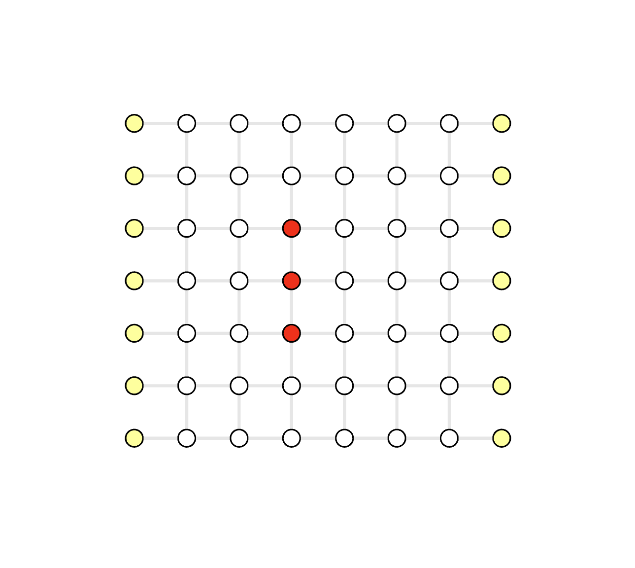
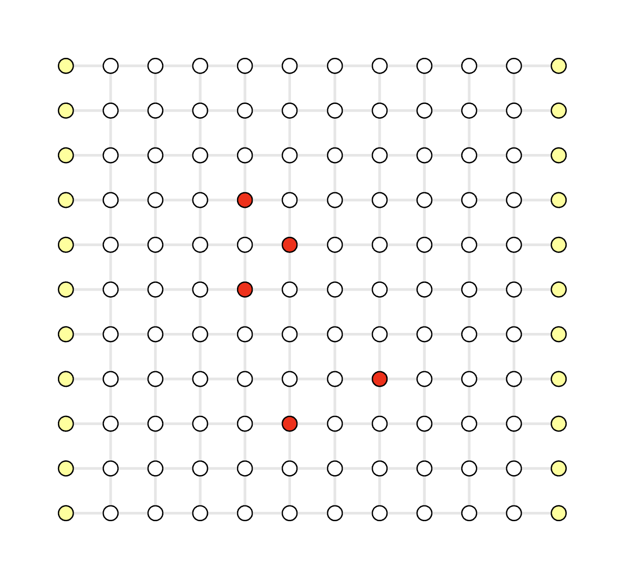
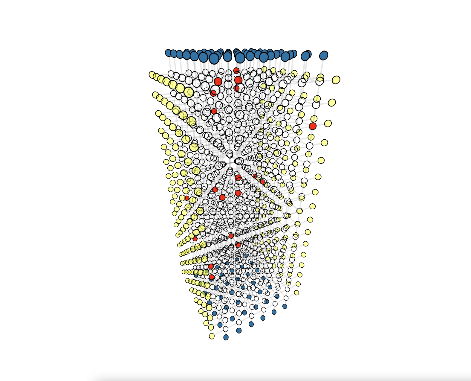
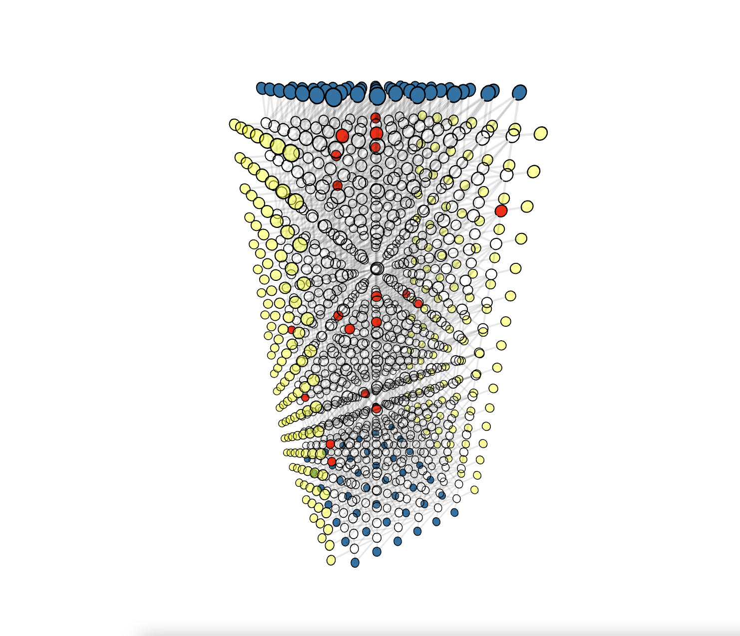
Demo
We highly suggest you watch through several demos here to get a sense of how the algorithm works. All our demos are captured from real algorithm execution. In fact, we're showing you the visualized debugger tool we wrote for fusion blossom. The demo is a 3D website and you can control the view point as you like.
For more details of why it finds an exact MWPM, please read our paper [coming soon 💪].
Click the demo image below to view the corresponding demo
Serial Execution
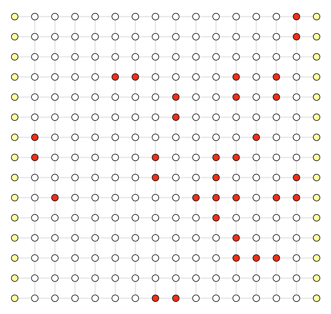
Parallel Execution (Shown in Serial For Better Visual)
Usage
Our code is written in Rust programming language for speed and memory safety, but it's hardly a easy language to learn. To make the decoder more accessible, we bind the library to Python and user can simply install the library using pip3 install fusion_blossom.
Here is an example for decode (you can run it by cloning the project and run python3 scripts/demo.py)
import fusion_blossom as fb

# create an example code
code = fb.CodeCapacityPlanarCode(d=11, p=0.05, max_half_weight=500)
initializer = code.get_initializer()  # the decoding graph structure (you can easily construct your own)
positions = code.get_positions()  # the positions of vertices in the 3D visualizer, optional

# randomly generate a syndrome according to the error model
syndrome = code.generate_random_errors(seed=1000)
with fb.PyMut(syndrome, "syndrome_vertices") as syndrome_vertices:
    syndrome_vertices.append(0)  # you can modify the syndrome vertices
print(syndrome)

# visualizer (optional for debugging)
visualizer = None
if True:  # change to False to disable visualizer for much faster decoding
    import os
    visualize_filename = fb.static_visualize_data_filename()
    visualizer = fb.Visualizer(filepath=visualize_filename, positions=positions)

solver = fb.SolverSerial(initializer)
solver.solve(syndrome, visualizer)  # enable visualizer for debugging
perfect_matching = solver.perfect_matching()
print(f"\n\nMinimum Weight Perfect Matching (MWPM):")
print(f"    - peer_matchings: {perfect_matching.peer_matchings}")  # Vec<(SyndromeIndex, SyndromeIndex)>
print(f"          = vertices: {[(syndrome_vertices[a], syndrome_vertices[b]) for a, b in perfect_matching.peer_matchings]}")
print(f"    - virtual_matchings: {perfect_matching.virtual_matchings}")  # Vec<(SyndromeIndex, VertexIndex)>
print(f"             = vertices: {[(syndrome_vertices[a], b) for a, b in perfect_matching.virtual_matchings]}")
subgraph = solver.subgraph(visualizer)
print(f"Minimum Weight Parity Subgraph (MWPS): {subgraph}\n\n")  # Vec<EdgeIndex>
solver.clear()  # clear is O(1) complexity, recommended for repetitive simulation

# view in browser
if visualizer is not None:
    fb.print_visualize_link(filename=visualize_filename)
    fb.helper.open_visualizer(visualize_filename, open_browser=True)
For parallel solver, it needs user to provide a partition strategy. Please wait for our paper for a thorough description of how partition works.
Evaluation
We use Intel(R) Xeon(R) Platinum 8375C CPU for evaluation, with 64 physical cores and 128 threads. Note that Apple m1max CPU has roughly 2x single-core decoding speed, but it has limited number of cores so we do not use data from m1max. By default, we test phenomenological noise model with $p$ = 0.005, code distance $d$ = 21, planar code with $d(d-1)$ = 420 $Z$ stabilizers, 100000 measurement rounds.
First of all, the number of partitions will effect the speed. Intuitively, the more partitions there are, the more overhead because fusing two partitions consumes more computation than solving them as a whole. But in practice, memory access is not always at the same speed. If cache cannot hold the data, then solving big partition may consume even more time than solving small ones. We test on a single-thread decoder, and try different partition numbers. At partition number = 1000, we get roughly the minimum decoding time of 3.4us per syndrome. This corresponds to each partition hosting 100 measurement rounds.

Given the optimal partition number of a single thread, we keep the partition number the same and try increasing the number of threads. Note that the partition number may not be optimal for large number of threads, but even in this case, we reach 41x speed up given 64 physical cores. The decoding time is pushed to 85ns per sydnrome or 1.0us per measurement round. This can catch up with the 1us measurement round of a superconducting circuit. Interestingly, we found that hyperthreading won't help much in this case, perhaps because this decoder is memory-bounded, meaning memory throughput is the bottleneck. Although the number of syndrome is only a small portion, they are randomly distributed so every time a new syndrome is given, the memory is almost always cold and incur large cache miss panelty.

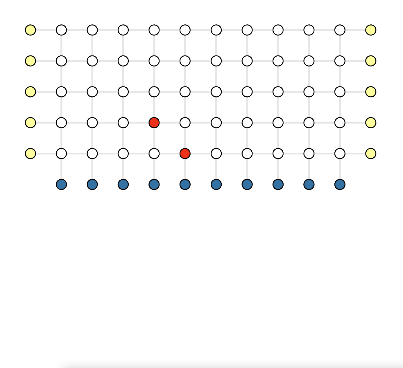
In order to understand the bottleneck of parallel execution, we wrote a visualization tool to display the execution windows of base partitions and fusion operations on multiple threads. Blue blocks is the base partition and green blocks is the fusion operation. Fusion operation only scales with the size of the fusion boundary and the depth of active partitions, irrelevant to the base partition's size. We'll study different partition and fusion strategies in our paper. Below shows the parallel execution on 24 threads. You can click the image and it will jump to this interactive visualization tool.

Interface
Sparse Decoding Graph and Integer Weights
The weights in QEC decoding graph are computed by taking the log of error probability, e.g. $w_e = \log{(1-p)/p}$ or roughly $w_e = -\log{p}$, we can safely use integers to save weights by e.g. multiplying the weights by 1e6 and truncate to nearest integer. In this way, the truncation error $\Delta w_e = 1$ of integer weights corresponds to relative error $\Delta p /{p}=10^{-6}$ which is small enough. Suppose physical error rate $p$ is in the range of a positive f64 variable (2.2e-308 to 1), the maximum weight is 7e7,which is well below the maximum value of a u32 variable (4.3e9). Since weights only sum up in our algorithm (no multiplication), u32 is large enough and accurate enough. By default we use usize which is platform dependent (usually 64 bits), but you can
We use integer also for ease of migrating to FPGA implementation. In order to fit more vertices into a single FPGA, it's necessary to reduce the resource usage for each vertex. Integers are much cheaper than floating-point numbers, and also it allows flexible trade-off between resource usage and accuracy, e.g. if all weights are equal, we can simply use a 2 bit integer.
Note that other libraries of MWPM solver like Blossom V also default to integer weights as well. Although one can change the macro to use floating-point weights, it's not recommended because "the code may even get stuck due to rounding errors".
Installation
Here is an example installation on Ubuntu20.04.
# install rust compiler and package manager
curl --proto '=https' --tlsv1.2 -sSf https://sh.rustup.rs | sh
# install build dependencies
sudo apt install build-essential
Tests
In order to test the correctness of our MWPM solver, we need a ground-truth MWPM solver. Blossom V is widely-used in existing MWPM decoders, but according to the license we cannot embed it in this library. To run the test cases with ground truth comparison or enable the functions like blossom_v_mwpm, you need to download this library at this website to a folder named blossomV at the root directory of this git repo.
wget -c https://pub.ist.ac.at/~vnk/software/blossom5-v2.05.src.tar.gz -O - | tar -xz
cp -r blossom5-v2.05.src/* blossomV/
rm -r blossom5-v2.05.src
Visualize
To start a server, run the following
cd visualize
npm install  # to download packages
# you can choose to render locally or to view it in a browser interactively
# interactive: open url using a browser (Chrome recommended)
node index.js <url> <width> <height>  # local render

# for example you can run the following command to get url
cd ..
cargo test visualize_paper_weighted_union_find_decoder -- --nocapture
TODOs
- support erasures in parallel solver
- optimize performance by statically handling object allocation without using Arc and Weak
- optimize scheduling of fusion operations and update data in README and MM2023 abstract
References
[1] Fowler, Austin G., et al. "Topological code autotune." Physical Review X 2.4 (2012): 041003.
[2] Criger, Ben, and Imran Ashraf. "Multi-path summation for decoding 2D topological codes." Quantum 2 (2018): 102.
[3] Fowler, Austin G., Adam C. Whiteside, and Lloyd CL Hollenberg. "Towards practical classical processing for the surface code: timing analysis." Physical Review A 86.4 (2012): 042313.
[4] Fowler, Austin G. "Minimum weight perfect matching of fault-tolerant topological quantum error correction in average $ O (1) $ parallel time." arXiv preprint arXiv:1307.1740 (2013).
[5] Higgott, Oscar. "PyMatching: A Python package for decoding quantum codes with minimum-weight perfect matching." ACM Transactions on Quantum Computing 3.3 (2022): 1-16.
[6] Delfosse, Nicolas, and Naomi H. Nickerson. "Almost-linear time decoding algorithm for topological codes." Quantum 5 (2021): 595.
[7] Wu, Yue. APS 2022 March Meeting Talk "Interpretation of Union-Find Decoder on Weighted Graphs and Application to XZZX Surface Code". Slides: https://us.wuyue98.cn/aps2022, Video: https://youtu.be/BbhqUHKPdQk
Release history Release notifications | RSS feed


Download files
Download the file for your platform. If you're not sure which to choose, learn more about installing packages.
Source Distributions
Built Distributions
Filter files by name, interpreter, ABI, and platform.
If you're not sure about the file name format, learn more about wheel file names.
Copy a direct link to the current filters
File details
Details for the file fusion_blossom-0.1.3-cp37-abi3-win_amd64.whl.
File metadata
- Download URL: fusion_blossom-0.1.3-cp37-abi3-win_amd64.whl
- Upload date:
- Size: 863.9 kB
- Tags: CPython 3.7+, Windows x86-64
- Uploaded using Trusted Publishing? No
- Uploaded via: twine/4.0.1 CPython/3.9.12
File hashes
| Algorithm | Hash digest | |
|---|---|---|
| SHA256 |
a083824491e1a1b585f69a3fa85d697d72e24e953bd589ecb0b7d5fb698fc6ae
|
|
| MD5 |
9816da681cf886a9ef773f11c5391c2b
|
|
| BLAKE2b-256 |
05692f5b4f98d4de1b883dc8781032c055c07ec12d0882b62680effb4c445145
|
File details
Details for the file fusion_blossom-0.1.3-cp37-abi3-win32.whl.
File metadata
- Download URL: fusion_blossom-0.1.3-cp37-abi3-win32.whl
- Upload date:
- Size: 796.9 kB
- Tags: CPython 3.7+, Windows x86
- Uploaded using Trusted Publishing? No
- Uploaded via: twine/4.0.1 CPython/3.9.12
File hashes
| Algorithm | Hash digest | |
|---|---|---|
| SHA256 |
70b88d5c1dcea17f7d423134080ac5c7f2e25a5f28cc498117c27c07baa936d0
|
|
| MD5 |
0fddd4155e1d7e830e3b8ba174d2c76e
|
|
| BLAKE2b-256 |
20cf3bdef7be5b54f70e76f029bafdbbcc4b91e024deab6c875fb1e878eeba4a
|
File details
Details for the file fusion_blossom-0.1.3-cp37-abi3-musllinux_1_1_x86_64.whl.
File metadata
- Download URL: fusion_blossom-0.1.3-cp37-abi3-musllinux_1_1_x86_64.whl
- Upload date:
- Size: 9.0 MB
- Tags: CPython 3.7+, musllinux: musl 1.1+ x86-64
- Uploaded using Trusted Publishing? No
- Uploaded via: twine/4.0.1 CPython/3.9.12
File hashes
| Algorithm | Hash digest | |
|---|---|---|
| SHA256 |
468ca65a06e04ef4ad423a27d131ca43b46c6bbf72b8eb2ffc5d4e6cfe21a6b6
|
|
| MD5 |
d6d5e9cb8489e67b87a1e8b3a9e739cc
|
|
| BLAKE2b-256 |
925fe86c8e7c8701ce6543dcfc6b061fa5c2c2ab34cbff95185be2e864d490ec
|
File details
Details for the file fusion_blossom-0.1.3-cp37-abi3-musllinux_1_1_aarch64.whl.
File metadata
- Download URL: fusion_blossom-0.1.3-cp37-abi3-musllinux_1_1_aarch64.whl
- Upload date:
- Size: 9.0 MB
- Tags: CPython 3.7+, musllinux: musl 1.1+ ARM64
- Uploaded using Trusted Publishing? No
- Uploaded via: twine/4.0.1 CPython/3.9.12
File hashes
| Algorithm | Hash digest | |
|---|---|---|
| SHA256 |
683faf1f33269ab6eeb0918992626b88fa985b1a34a1afb56193a02f61a2a9a8
|
|
| MD5 |
e3c3b31967db5c7542ef5d4a92540d8d
|
|
| BLAKE2b-256 |
32de6b752f7c7004585615d254c36a2a35991613070d24653540c32814a44c9d
|
File details
Details for the file fusion_blossom-0.1.3-cp37-abi3-manylinux_2_17_x86_64.manylinux2014_x86_64.whl.
File metadata
- Download URL: fusion_blossom-0.1.3-cp37-abi3-manylinux_2_17_x86_64.manylinux2014_x86_64.whl
- Upload date:
- Size: 9.0 MB
- Tags: CPython 3.7+, manylinux: glibc 2.17+ x86-64
- Uploaded using Trusted Publishing? No
- Uploaded via: twine/4.0.1 CPython/3.9.12
File hashes
| Algorithm | Hash digest | |
|---|---|---|
| SHA256 |
22aa585223df111cbfd560f0d08b0eeac61ec02f93b16b25854dad502c9bca7d
|
|
| MD5 |
1d16fc7f3d6195e6042961b28391eca3
|
|
| BLAKE2b-256 |
c3d38016d1697d033e2149e376a611fdbe1a48291f754aa5393eb5a6bd89d352
|
File details
Details for the file fusion_blossom-0.1.3-cp37-abi3-manylinux_2_17_aarch64.manylinux2014_aarch64.whl.
File metadata
- Download URL: fusion_blossom-0.1.3-cp37-abi3-manylinux_2_17_aarch64.manylinux2014_aarch64.whl
- Upload date:
- Size: 9.0 MB
- Tags: CPython 3.7+, manylinux: glibc 2.17+ ARM64
- Uploaded using Trusted Publishing? No
- Uploaded via: twine/4.0.1 CPython/3.9.12
File hashes
| Algorithm | Hash digest | |
|---|---|---|
| SHA256 |
81358499946eb1806cde2cf6abe7d4a92917fd837118e5f9b7c7313597dc0834
|
|
| MD5 |
d2c9d40c28f8e54acecd34229833d3e3
|
|
| BLAKE2b-256 |
3e227570c5100c08604c4128db57d37ebf8ea50775ea3096c31bcf2882140991
|
File details
Details for the file fusion_blossom-0.1.3-cp37-abi3-macosx_10_9_x86_64.macosx_11_0_arm64.macosx_10_9_universal2.whl.
File metadata
- Download URL: fusion_blossom-0.1.3-cp37-abi3-macosx_10_9_x86_64.macosx_11_0_arm64.macosx_10_9_universal2.whl
- Upload date:
- Size: 2.3 MB
- Tags: CPython 3.7+, macOS 10.9+ universal2 (ARM64, x86-64), macOS 10.9+ x86-64, macOS 11.0+ ARM64
- Uploaded using Trusted Publishing? No
- Uploaded via: twine/4.0.1 CPython/3.9.12
File hashes
| Algorithm | Hash digest | |
|---|---|---|
| SHA256 |
4559e2b25965abff0735e5830bf0c99251027c39f19093e495d5ec54c3e19b5b
|
|
| MD5 |
31dac436bcdaa3476214d77db978f8b2
|
|
| BLAKE2b-256 |
98be947d6640cd7b84739cd64348c557d48f91c2dd7b24e37995ac2dc42a8133
|


