Utilities for masking, contour tracing, and geocontour construction with gridded geographic data

Project description
 geocontour
Utilities for masking, contour tracing, and geocontour construction with gridded geographic data.


Installation
pip install geocontour
or
pip install git+https://github.com/benkrichman/geocontour.git@main
To run a full test of internal functions (minus cartopy features):
geocontour.tests.full()
Documentation
Find the full documentation hosted here.
Citation
If geocontour played a significant role in your work and you would like to cite it, the following is suggested (APA):
Krichman, B. (2023). geocontour (Version 1.3.1) [Computer Software]. https://doi.org/10.5281/zenodo.7402714
Bibtex:
@software{geocontour,
author={Krichman, Benjamin},
doi={10.5281/zenodo.7402714},
license={MIT},
month={5},
year={2023},
title={{geocontour}},
url={https://github.com/benkrichman/geocontour},
version={1.3.1},
note = {Computer Software}
}
Features
Masks
Selectable/tunable criteria for masks created from input boundary coordinates
- cell center (multiple methods with variable precision)
- node ratio (multiple methods with variable precision)
- area ratio
Useful mask operators
- return mask connectivity (and null connectivity)
- return mask edge cells
- return mask vertex points
Contours
Implements 6 existing algorithms for contour tracing, and two improvements on known algorithms
- square tracing (a.k.a. simple boundary follower/Papert's turtle algorithm) 12345
- moore neighbor tracing 15
- improved moore neighbor tracing (capturing inside corners)
- pavlidis tracing 16
- improved pavlidis tracing (capturing inside corners)
- modified simple boundary follower 782
- improved simple boundary follower 784
- fast representative tracing 4
Tuning of contours created from tracing input masks
- trace direction
- selectable and adjustable stopping conditions
- automatic or manual selection of starting cell
- selectable connection type (cell to cell or cell edge to cell center)
- simplification of output contour (removal of repeating cells)
- selectable contour closure
- usable for an associated lat/lon grid or on a non-specified grid
Useful contour operators
- return full search path for a contour trace
- return cell neighbors with connectivity and directional input
- return starting cell for contour tracing and check that starting cells work for a given algorithm
- return visually improved contour search
Geocontours
From an input contour, create a closed geospatial contour with calculated segment lengths and outward unit vectors (for example: useful in calculating flux across a bounding surface from a geospatial data set)
Options for tuning criteria of geocontours created from input contours
- selectable connection type (cell to cell or cell edge to cell center)
- optionally simplify geocontours at the cell level to shorten and improve compute times in practical applications
Timing
Timing modules for easy comparison between mask search methods or contour tracing algorithms using timeit.
Note that in mask search and contour tracing care has been taken to implement algorithms in a fast and efficient manner through utilization of shapely and matplotlib builtins and through numpy vectorization where possible. However, not everything is speed optimized where optimization would necessitate significantly more complexity or utilization of external low level libraries or custom functions. The timing modules exist for intercomparison amongst methods, but also for giving users a reasonable expectation of performance.
Visualization
Easy and semi-automated plotting function for visualization of boundaries/masks/contours/contour searches/geocontours
- buffers
- grid overlay
- mask/contour cell visibility
- directional indicators for contours and contour searches
- outward unit vector indicators for geocontours
- automatic calculation of feature size and output resolution
- display of natural features or political boundaries (optional with cartopy installed)
- selectable marker/line/arrow/cell size/color/style
- optional transparency mode for presentation/publication use
Example Use Case
*to reconstruct these examples use (or view)
geocontour.examples.small()
geocontour.examples.large()
mask search
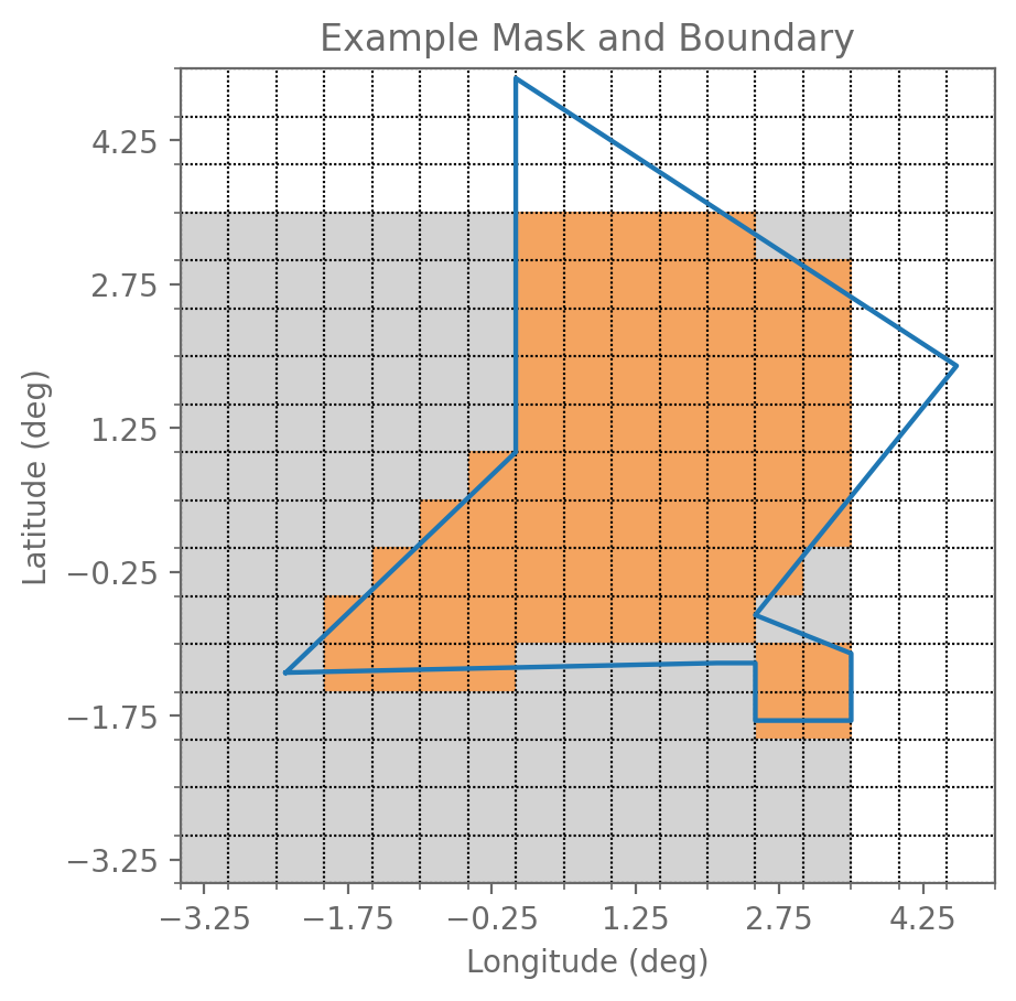
Given a series of lat/lon points constituting a geographical boundary, and a set of gridded data on a lat/lon grid, find an appropriate mask to select gridded data within the boundary:
Use the 'area' approach to mask calculation, defaulting to selection of all cells for which 50% or greater falls withing the boundary. Note that boundary falls outside gridded data bounds at some points and those cells inside the boundary but outside the gridded data bounds are not included in the mask.
mask=geocontour.masksearch.area(latitudes,longitudes,boundary)
geocontour.output.plot(latitudes,longitudes,boundary=boundary,mask=mask,title='Example Mask and Boundary',outname='example_small_boundary+mask',outdpi='indep')
contour trace
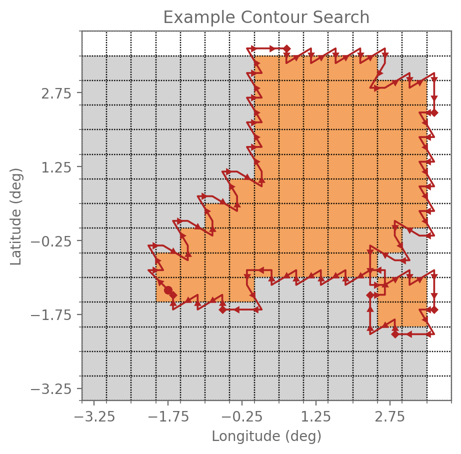
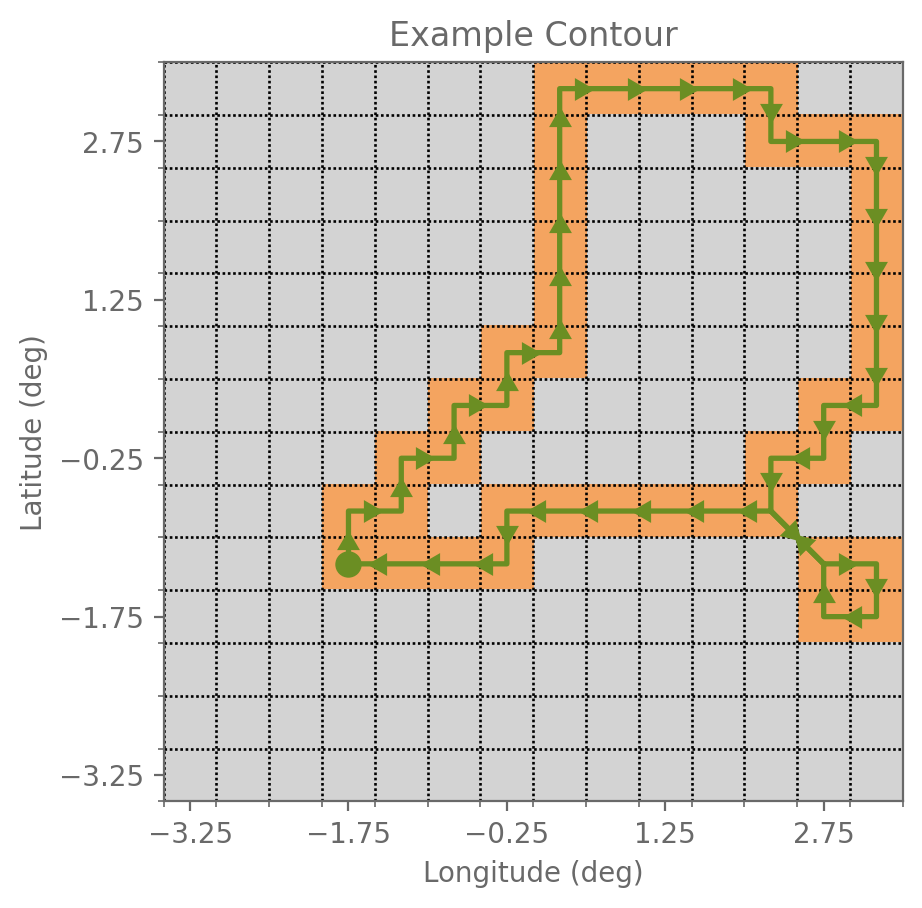
Given the previously calculated mask, find the outer edge using a contour tracing algorithm:
Use the improved Pavlidis algorithm to trace the contour. Note that the contoursearch plot shows the start cell as a circle, directional arrows for each segment, and diamonds where cells are consecutively and repeatedly searched. In the case of the pavlidis algorithm these diamonds show where the orientation turned 90 degrees. Similarly the contour plot uses a circle to mark the start cell and arrows to signify direction.
contour,contoursearch=geocontour.contourtrace.pavlidis_imp(mask,latitudes,longitudes)
geocontour.output.plot(latitudes,longitudes,mask=mask,contoursearch=contoursearch,title='Example Contour Search',outname='example_small_contoursearch',outdpi='indep')
geocontour.output.plot(latitudes,longitudes,contour=contour,cells='contour',title='Example Contour',outname='example_small_contour',outdpi='indep')
construct geocontour
Given the previously calculated contour, construct the geocontour to determine contour segment lengths and outward normal vectors:
Use the build function of geocontour to construct the geocontour. Note that in the second plot the 'simplify' option is used, combining cells with multiple visits into single segments exactly equal to the vector combination of segments in the cell. The directional information contained in the contour has been discarded, and in the case of simplification may not be extractable from the geocontour.
geocontour=geocontour.build(contour,latitudes,longitudes)
geocontour_simp=geocontour.build(contour,latitudes,longitudes,simplify=True)
geocontour.output.plot(latitudes,longitudes,geocontour=geocontour,buffer='on',title='Example Geocontour',outname='example_small_geocontour',outdpi='indep')
geocontour.output.plot(latitudes,longitudes,geocontour=geocontour_simp,buffer='on',title='Example Geocontour - Simplified',outname='example_small_geocontour_simp',outdpi='indep')
project geocontour against map features
Given a large geocontour (in this case, the Mississippi River Basin) project against natural features and political borders (requires cartopy):
geocontour.output.plot(latitudes,longitudes,geocontour=geocontour,title='Example Geocontour\nMississippi River Basin',outname='example_large_geocontour+natfeat',features='natural')
geocontour.output.plot(latitudes,longitudes,geocontour=geocontour,title='Example Geocontour\nMississippi River Basin',outname='example_large_geocontour+bordfeat',features='borders')
-
Ghuneim, A.G. (2000). Contour Tracing. McGill University. https://www.imageprocessingplace.com/downloads_V3/root_downloads/tutorials/contour_tracing_Abeer_George_Ghuneim/alg.html ↩ ↩2 ↩3
-
Gose, E., Johnsonbaugh, R., & Jost, S. (1996). Pattern recognition and image analysis. Prentice Hall PTR. ↩ ↩2
-
Papert, S. (1973). Uses of Technology to Enhance Education (No. 298; Artificial Intelligence). Massachusetts Institute of Technology. https://dspace.mit.edu/handle/1721.1/6213 ↩
-
Seo, J., Chae, S., Shim, J., Kim, D., Cheong, C., & Han, T.-D. (2016). Fast Contour-Tracing Algorithm Based on a Pixel-Following Method for Image Sensors. Sensors, 16(3), 353. https://doi.org/10.3390/s16030353 ↩ ↩2 ↩3
-
Toussaint, G.T. (2010). Grids Connectivity and Contour Tracing [Lesson Notes]. McGill University. http://www-cgrl.cs.mcgill.ca/~godfried/teaching/mir-reading-assignments/Chapter-2-Grids-Connectivity-Contour-Tracing.pdf ↩ ↩2
-
Pavlidis, T. (1982) Algorithms for Graphics and Image Processing. Computer Science Press, New York, NY. https://doi.org/10.1007/978-3-642-93208-3 ↩
-
Cheong, C.-H., & Han, T.-D. (2006). Improved Simple Boundary Following Algorithm. Journal of KIISE: Software and Applications, 33(4), 427–439. https://koreascience.kr/article/JAKO200622219415761.pdf ↩ ↩2
-
Cheong, C.-H., Seo, J., & Han, T.-D. (2006). Advanced Contour Tracing Algorithms based on Analysis of Tracing Conditions. Proceedings of the 33rd KISS Fall Conference, 33, 431–436. https://koreascience.kr/article/CFKO200614539217302.pdf ↩ ↩2


Download files
Download the file for your platform. If you're not sure which to choose, learn more about installing packages.
Source Distribution
Built Distribution
Filter files by name, interpreter, ABI, and platform.
If you're not sure about the file name format, learn more about wheel file names.
Copy a direct link to the current filters
File details
Details for the file geocontour-1.3.1.tar.gz.
File metadata
- Download URL: geocontour-1.3.1.tar.gz
- Upload date:
- Size: 10.3 MB
- Tags: Source
- Uploaded using Trusted Publishing? No
- Uploaded via: twine/4.0.2 CPython/3.10.10
File hashes
| Algorithm | Hash digest | |
|---|---|---|
| SHA256 |
56b52c60a4100fe5f1c1ba2d0a389281f0f5b4edbd334ac93cac5a178a5410af
|
|
| MD5 |
2b28a3205961ecb7d61d52b8b2ee481a
|
|
| BLAKE2b-256 |
71544ddc1a964f85d9e851ca4af4209c27ec5547762ec81ba13fab0765dcc93b
|
File details
Details for the file geocontour-1.3.1-py3-none-any.whl.
File metadata
- Download URL: geocontour-1.3.1-py3-none-any.whl
- Upload date:
- Size: 92.2 kB
- Tags: Python 3
- Uploaded using Trusted Publishing? No
- Uploaded via: twine/4.0.2 CPython/3.10.10
File hashes
| Algorithm | Hash digest | |
|---|---|---|
| SHA256 |
47594312523e951835a5adc6c4653886cc1d7f69738445201e64dec300da2846
|
|
| MD5 |
f21f3575da1635a48e05c4a0793b1ed7
|
|
| BLAKE2b-256 |
b6902318c722a348f56c55e72d481513a745f01c778d20deddc89dbba7e3a667
|


