Python interface for Gillespie-style biochemical simulations
Project description

GillesPy2 is a Python 3 package for stochastic simulation of biochemical systems. It offers an object-oriented approach for creating mathematical models of biological systems, as well as a variety of methods for performing time simulation of those models. The methods include the Gillespie direct method (SSA), several variant stochastic simulation methods including tau-Leaping, and numerical integration of ODEs. The solvers support a variety of user environments, with optimized code for C++, and NumPy. GillesPy2 also supports SBML.
 PLEASE REGISTER AS A USER, so that we can prove GillesPy2 has many users when we seek funding to support development. GillesPy2 is part of the StochSS project.
|
Table of contents
- Table of contents
- Installation
- Usage
- Getting help
- Contributing
- License
- Authors and history
- Acknowledgments
Installation
GillesPy2 can be installed on your computer using different methods, as described below.
Using PyPI
On Linux, macOS, and Windows operating systems, you should be able to install GillesPy2 with pip. Please review the official pip documentation for installation instructions and additional information.
Then, to install GillesPy2 from the Python package repository, run the following command:
python3 -m pip install gillespy2 --user --upgrade
Using the source code repository
As an alternative to getting it from PyPI, you can instruct pip to install GillesPy2 directly from the GitHub repository:
python3 -m pip install https://github.com/StochSS/GillesPy2/archive/main.zip --user --upgrade
As a final alternative, you can first use git to clone a copy of the GillesPy2 source tree from the GitHub repository to your local computer disk, and then install GillesPy2 using that copy:
git clone https://github.com/StochSS/GillesPy2.git
cd GillesPy2
python3 -m pip install  .  --user --upgrade
NOTE: to import/export SMBL, libSBML must be installed. It is not installed by default with GillesPy2. To include libSBML in the installation of GillesPy2 use pip install gillespy2[sbml]. If GillesPy2 is already installed use pip install python_libSBML.
Usage
GillesPy2 provides simple object-oriented abstractions for defining a model of a biochemical system and simulating that model using efficient stochastic simulation algorithms. The basic steps to use GillesPy2 are:
- Create a
GillesPy2.Modelcontaining molecular species, parameters, and reactions (or import it from an SBML file) - Invoke the model's
.run()method.
The run() method can be customized using keyword arguments to select different solvers, random seed, data return type and more. For more detailed examples on how to use GillesPy2, please see the Getting Started Jupyter notebook contained in the examples subdirectory.
Simple example to illustrate the use of GillesPy2
Dimerization is a process in which two molecules of some molecular species (known as a "monomer" in this situation – let's call it "M" for short) come together to create a new molecule (call it "D"), but do so in a way that is reversible, meaning the combined structure can also decay or dissociate back into "M". A simple model of the dimerization process represents it as two reactions: a reaction in which one molecule of "M" reacts with another molecule of "M" to form one new molecule ("D"), and another reaction in which a molecule of "D" breaks apart into two molecules of "M". In terms of biochemical reactions, it looks like this (where kc and kd represent the rate constants for creation and dissociation of the dimer, respectively; M represents the number of molecules of "M"; and D is the number of molecules of "D"):
kc
2 M ⟷ D
kd
In GillesPy2, a model is expressed as an object. Components, such as the reactions, molecular species, and characteristics such as the time span for simulation, are all defined within the model. The following Python code represents our dimerization model using GillesPy2's facility:
def create_dimerization(parameter_values=None):
    # First call the gillespy2.Model initializer.
    model = gillespy2.Model(name='Dimerization')

    # Define parameters for the rates of creation and dissociation.
    k_c = gillespy2.Parameter(name='k_c', expression=0.005)
    k_d = gillespy2.Parameter(name='k_d', expression=0.08)
    model.add_parameter([k_c, k_d])

    # Define variables for the molecular species representing M and D.
    m = gillespy2.Species(name='monomer', initial_value=30)
    d = gillespy2.Species(name='dimer',   initial_value=0)
    model.add_species([m, d])

    # The list of reactants and products for a Reaction object are each a
    # Python dictionary in which the dictionary keys are Species objects
    # and the values are stoichiometries of the species in the reaction.
    r_c = gillespy2.Reaction(name="r_creation", rate=k_c, reactants={m:2}, products={d:1})
    r_d = gillespy2.Reaction(name="r_dissociation", rate=k_d, reactants={d:1}, products={m:2})
    model.add_reaction([r_c, r_d])

    # Set the timespan for the simulation.
    tspan = gillespy2.TimeSpan.linspace(t=100, num_points=101)
    model.timespan(tspan)
    return model
Given the model creation function above, the model can be simulated by first instantiating the model object, and then invoking the run() method on the object. The following code will run the model 10 times to produce 10 sample trajectories:
model = create_dimerization()
results = model.run(number_of_trajectories=10)
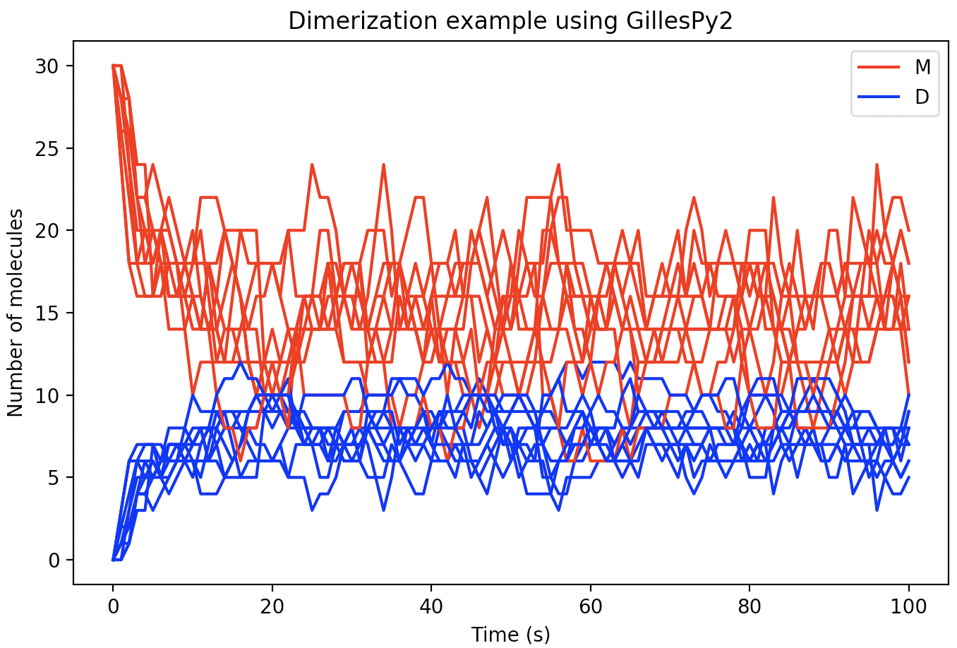
The results are then stored in a class Results object for single trajectory or for multiple trajectories. Results can be plotted with matplotlib using plot() or in plotly (offline) using plotplotly(). For additional plotting options such as plotting from a selection of species, or statistical plotting, please see the documentation.:
results.plot()

Alternatively, the results object inherits python-builtin UserDict for single trajectories, and UserList for multiple trajectories. Results can be plotted easily using any plotting library such as matplotlib as shown below:
for index in range(0, 10):
    trajectory = results[index]
    plt.plot(trajectory['time'], trajectory['monomer'], 'r')
    plt.plot(trajectory['time'], trajectory['dimer'],   'b')
With a few additional Python matplotlib commands to create figure labels and such, we end up with a plot like this:

Getting help
GillesPy2's online documentation provides more details about using the software. If you find any problem with GillesPy2 or the documentation, please report it using the GitHub issue tracker for this repository. You can also contact Dr. Brian Drawert directly with questions and suggestions.
Contributing
We would be happy to receive your help and participation with enhancing GillesPy2! The UML class diagram and Pynsource UML class model may help you familiarize yourself with the existing code. Please follow the guidelines described in CONTRIBUTING.md.
New developments happen primarily in the develop branch. New releases are put in the main branch.
| Main Branch | Develop Branch | Test Coverage | Maintainability |
|---|---|---|---|
 |
 |
 |
 |
License
GillesPy2 is licensed under the GNU General Public License version 3. Please see the file LICENSE for more information.
Authors and history
- Dr. Brian Drawert
- Dr. Kevin Sanft
- Ghilman Brock
- Eliot Dixon
- Dalton Nickerson
- Sean Matthew
- Matthew Geiger
- Kassidy Hall
- W.R. Jackson
- Samuel Hodges
- Emma Weisgerber
- Adrien Coulier
- Mike Hucka
- Fredrik Wrede
- Prashant Singh
- Bryan Rumsey
- Mason Kidwell
- Jesse Reeve
- Fin Carter
- Ethan Green
- Josh Cooper
- Matthew Dippel
- Joshua Fisher-Caudill
Acknowledgments
This work has been funded by National Institutes of Health (NIH) NIBIB Award No. 2R01EB014877-04A1.
GillesPy2 uses numerous open-source packages, without which it would have been effectively impossible to develop this software with the resources we had. We want to acknowledge this debt. In alphabetical order, the packages are:
- Jupyter – web application for creating documents containing code, visualizations and narrative text
- libSBML – a library for reading, writing, and manipulating SBML content
- lxml – an XML parsing library for Python
- MatplotLib – Python plotting library
- Plotly – Graphing library for making interactive, publication-quality graphs
- Numpy – the fundamental package for scientific computing with Python
- Scipy – Python-based ecosystem of open-source software for mathematics, science, and engineering
Finally, we are grateful for institutional resources made available by the University of North Carolina at Asheville, the University of California at Santa Barbara, Uppsala University, and the California Institute of Technology.
Project details
Release history Release notifications | RSS feed
Download files
Download the file for your platform. If you're not sure which to choose, learn more about installing packages.
Source Distribution
Built Distribution
Filter files by name, interpreter, ABI, and platform.
If you're not sure about the file name format, learn more about wheel file names.
Copy a direct link to the current filters
File details
Details for the file gillespy2-1.8.3.tar.gz.
File metadata
- Download URL: gillespy2-1.8.3.tar.gz
- Upload date:
- Size: 313.9 kB
- Tags: Source
- Uploaded using Trusted Publishing? No
- Uploaded via: twine/5.1.1 CPython/3.9.6
File hashes
| Algorithm | Hash digest | |
|---|---|---|
| SHA256 |
8eed59b5ba12614225a7fdb42ebb72e461bbd3a1e23947fef359e16eeaed845f
|
|
| MD5 |
1c4ba298e9ea65a1115e90eda98d4f37
|
|
| BLAKE2b-256 |
02b0c13e3c4f2f66412b4603234e9c2dfd6bec68926c89b40d8339479cdbcd11
|
File details
Details for the file gillespy2-1.8.3-py3-none-any.whl.
File metadata
- Download URL: gillespy2-1.8.3-py3-none-any.whl
- Upload date:
- Size: 398.9 kB
- Tags: Python 3
- Uploaded using Trusted Publishing? No
- Uploaded via: twine/5.1.1 CPython/3.9.6
File hashes
| Algorithm | Hash digest | |
|---|---|---|
| SHA256 |
7907880eaf5e542ca1efad598f5d59d306f01355262ef35f9217a49d825692f0
|
|
| MD5 |
b1841095509ed623be46d57fb3c99406
|
|
| BLAKE2b-256 |
ba58e2bc558d9bb5b9745cb847833cc817318fa0549bd62af566e5a13d392d87
|


