Measures the resource utilization of a specific process over time

Project description
Overview
Measures the resource utilization of a specific process over time.
Also measures the utilization/saturation of system-wide resources: this helps putting the process-specific metrics into context.
Built for Linux. Windows and Mac OS support might come.
For a list of the currently supported metrics see below.
The name, Göffel, is German for spork:

Convenient, right?
Highlights
- High sampling rate: the default sampling interval of
0.5 smakes narrow spikes visible. - Can monitor a program subject to process ID changes (for longevity experiments where the monitored process occasionally restarts, for instance as of fail-over scenarios).
- Can run indefinitely. Has predictable disk space requirements (output file rotation and retention policy).
- Keeps your data organized: the time series data is written into a structured HDF5 file annotated with relevant metadata (also including program invocation time, system hostname, a custom label, the Goeffel software version, and others).
- Interoperability: output files can be read with any HDF5 reader such as PyTables and especially with pandas.read_hdf(). See tips and tricks.
- Values measurement correctness very highly (see technical notes).
- Comes with a data plotting tool separate from the data acquisition program.
Download & installation
The latest Goeffel release can be downloaded and installed from PyPI, via pip:
$ pip install goeffel
pip can also install the latest development version of Goeffel:
$ pip install git+https://github.com/jgehrcke/goeffel
CLI tutorial
goeffel: data acquisition
Invoke Goeffel with the --pid <pid> argument if the process ID of the target process is known.
In this mode, goeffel stops the measurement and terminates itself once the process with the given ID goes away. Example:
$ goeffel --pid 29019

[... snip ...]

190809-15:46:57.914 INFO: Updated HDF5 file: wrote 20 sample(s) in 0.01805 s

[... snip ...]

190809-15:56:13.842 INFO: Cannot inspect process: process no longer exists (pid=29019)
190809-15:56:13.843 INFO: Wait for producer buffer to become empty
190809-15:56:13.843 INFO: Wait for consumer process to terminate
190809-15:56:13.854 INFO: Updated HDF5 file: wrote 13 sample(s) in 0.01077 s
190809-15:56:13.856 INFO: Sample consumer process terminated
For measuring beyond the process lifetime use --pid-command <command>.
In the following example, I use the pgrep utility is for discovering the newest stress process:
$ goeffel --pid-command 'pgrep stress --newest'

[... snip ...]

190809-15:47:47.337 INFO: New process ID from PID command: 25890

[... snip ...]

190809-15:47:57.863 INFO: Updated HDF5 file: wrote 20 sample(s) in 0.01805 s
190809-15:48:06.850 INFO: Cannot inspect process: process no longer exists (pid=25890)
190809-15:48:06.859 INFO: PID command returned non-zero

[... snip ...]

190809-15:48:09.916 INFO: PID command returned non-zero
190809-15:48:10.926 INFO: New process ID from PID command: 28086
190809-15:48:12.438 INFO: Updated HDF5 file: wrote 20 sample(s) in 0.01013 s
190809-15:48:22.446 INFO: Updated HDF5 file: wrote 20 sample(s) in 0.01062 s

[... snip ...]
In this mode, goeffel runs forever until manually terminated via SIGINT or SIGTERM.
Process ID changes are detected by periodically running the discovery command until it returns a valid process ID on stdout.
This is useful for longevity experiments where the monitored process occasionally restarts, for instance as of fail-over scenarios.
goeffel-analysis: data inspection and visualization
Note: goeffel-analysis provides an opinionated and limited approach to visualizing data. For advanced and thorough data analysis I recommend building a custom (maybe even ad-hoc) data analysis pipeline using pandas and matplotlib, or using the tooling of your choice.
Also note: The command line interface provided by goeffel-analysis,
especially for the plot commands, might change in the future. Suggestions for
improvement are welcome, of course.
goeffel-analysis inspect:
Use goeffel-analysis inspect <path-to-HDF5-file> for inspecting the contents
of a Goeffel output file. Example:
$ goeffel-analysis inspect mwst18-master1-journal_20190801_111952.hdf5
Measurement metadata:
  System hostname: int-master1-mwt18.foo.bar
  Invocation time (local): 20190801_111952
  PID command: pgrep systemd-journal
  PID: None
  Sampling interval: 1.0 s

Table properties:
  Number of rows: 24981
  Number of columns: 38
  Number of data points (rows*columns): 9.49E+05
  First row's (local) time: 2019-08-01T11:19:53.613377
  Last  row's (local) time: 2019-08-01T18:52:49.954582
  Time span: 7h 32m 56s

Column names:
  unixtime
  ... snip ...
  system_mem_inactive
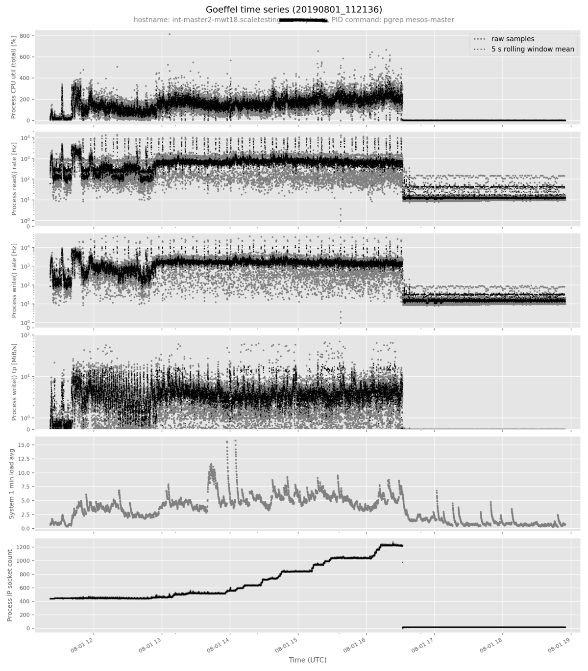
goeffel-analysis plot: quickly plot data from a single time series file
The goeffel-analysis plot <path-to-hdf5-file> command plots a pre-selected
set of metrics in an opinionated way. More metrics can be added to the plot with
the --metric <metric-name> option. Example command:
goeffel-analysis plot \
  mwst18-master2-mesosmaster_20190801_112136.hdf5 \
  --metric proc_num_ip_sockets_open
Example output figure:
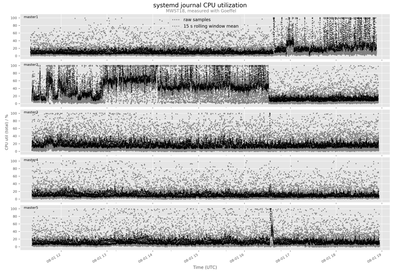
goeffel-analysis flexplot: generic plot command
This command can be used for example for comparing multiple time series.
Say you have monitored the same program across multiple replicas in a distributed system and would like to compare the time evolution of a certain metric across these replicas.
Then the goeffel-analysis flexplot command is here to help, invoked with multiple --series arguments:
$ goeffel-analysis flexplot \
  --series mwst18-master1-journal_20190801_111952.hdf5 master1 \
  --series mwst18-master2-journal_20190801_112136.hdf5 master2 \
  --series mwst18-master3-journal_20190801_112141.hdf5 master3 \
  --series mwst18-master4-journal_20190801_112151.hdf5 master4 \
  --series mwst18-master5-journal_20190801_112157.hdf5 master5 \
  --column proc_cpu_util_percent_total \
      'CPU util (total) / %' \
      'systemd journal CPU utilization ' 15 \
  --subtitle 'MWST18, measured with Goeffel' \
  --legend-loc 'upper center'
Example output figure:
Background and details
Prior art
This was born out of a need for solid tooling. We started with pidstat from
sysstat, launched as
pidstat -hud -p $PID 1 1. We found that it does not properly account for
multiple threads running in the same process and that various issues in that
regard exist in this program across various versions (see
here,
here, and
here).
The program cpustat open-sourced by Uber has a delightful README about the general measurement methodology and overall seems to be a great tool. However, it seems to be optimized for interactive usage (whereas we were looking for a robust measurement program which can be pointed at a process and then be left unattended for a significant while) and there does not seem to be a well-documented approach towards persisting the collected time series data on disk for later inspection.
The program psrecord (which effectively wraps psutil) has a similar fundamental approach as Goeffel; it however only measures few metrics, and it does not have a clear separation of concerns between persisting the data to disk, performing the measurement itself, and analyzing/plotting the data.
Technical notes
-
The core sampling loop does little work besides the measurement itself: it writes each sample to a queue. A separate process consumes this queue and persists the time series data to disk, for later inspection. This keeps the sampling rate predictable upon disk write latency spikes, or generally upon backpressure. This matters especially in cloud environments where we sometimes see fsync latencies of multiple seconds.
-
The sampling loop is (supposed to be, feedback welcome) built so that timing-related systematic measurement errors are minimized.
-
Goeffel tries to not asymmetrically hide measurement uncertainty. For example, you might see it measure a CPU utilization of a single-threaded process slightly larger than 100 %. That's simply the measurement error. In related tooling such as
sysstatit seems to be common practice to asymmetrically hide measurement uncertainty by capping values when they are known to in theory not exceed a certain threshold (example). -
goeffelmust be run withrootprivileges. -
The value
-1has a special meaning for some metrics (NaN, which cannot be represented properly in HDF5). Example: A disk write latency of-1 msmeans that no write happened in the corresponding time interval. -
The highest meaningful sampling rate is limited by the kernel's timer and bookkeeping system.
Measurands
Measurand is a word! This section attempts to describe the individual data columns ("metrics"), their units, and their meaning. There are four main categories:
Timestamps
unixtime, isotime_local, monotime
The timestamp corresponding to the right boundary of the sampled time interval.
-
unixtimeencodes the wall time. It is a canonical Unix timestamp (seconds since epoch, double-precision floating point number); with sub-second precision and no timezone information. This is compatible with a wide range of tooling and therefore the general-purpose timestamp column for time series analysis (also see How to convert theunixtimecolumn into apandas.DatetimeIndex). Note: this is subject to system clock drift. In extreme case, this might go backward, have discontinuities, and be a useless metric. In that case, themonotimemetric helps (see below). -
isotime_localis a human-readable version of the same timestamp as stored inunixtime. It is a 26 character long text representation of the local time using an ISO 8601 notation (and therefore also machine-readable). Likeunixtimethis metric is subject to system clock drift and might become pretty useless in extreme cases. -
monotimeis based on a so-called monotonic clock source that is not subject to (accidental or well-intended) system clock drift. This column encodes most accurately the relative time difference between any two samples in the time series. The timestamps encoded in this column only make sense relative to each other; the difference between any two values in this column is a wall time difference in seconds, with sub-second precision.
Process-specific metrics
proc_pid
The process ID of the monitored process. It can change if Goeffel was invoked
with the --pid-command option.
Momentary state at sampling time.
proc_cpu_util_percent_total
The CPU utilization of the process in percent.
Mean over the past sampling interval.
If the inspected process is known to contain just a single thread then this can still sometimes be larger than 100 % as of measurement errors. If the process runs more than one thread then this can go far beyond 100 %.
This is based on the sum of the time spent in user space and in kernel space.
For a more fine-grained picture the following two metrics are also available:
proc_cpu_util_percent_user, and proc_cpu_util_percent_system.
proc_cpu_id
The ID of the CPU that this process is currently running on.
Momentary state at sampling time.
proc_ctx_switch_rate_hz
The rate of (voluntary and
involuntary) context switches in Hz.
Mean over the past sampling interval.
proc_num_threads
The number of threads in the process.
Momentary state at sampling time.
proc_num_ip_sockets_open
The number of sockets currently being open. This includes IPv4 and IPv6 and does not distinguish between TCP and UDP, and the connection state also does not matter.
Momentary state at sampling time.
proc_num_fds
The number of file descriptors currently opened by this process.
Momentary state at sampling time.
proc_disk_read_throughput_mibps and proc_disk_write_throughput_mibps
The disk I/O throughput of the inspected process, in MiB/s.
Based on Linux' /proc/<pid>/io rchar and wchar. Relevant
Linux kernel documentation (emphasis mine):
rchar: The number of bytes which this task has caused to be read from storage. This is simply the sum of bytes which this process passed to read() and pread(). It includes things like tty IO and it is unaffected by whether or not actual physical disk IO was required (the read might have been satisfied from pagecache).
wcar: The number of bytes which this task has caused, or shall cause to be written to disk. Similar caveats apply here as with rchar.
Mean over the past sampling interval.
proc_disk_read_rate_hz and proc_disk_write_rate_hz
The rate of read/write system calls issued by the process as inferred from the
Linux /proc file system. The relevant syscr/syscw counters are as of now
only documented with "read I/O operations, i.e. syscalls like read() and
pread()" and "write I/O operations, i.e. syscalls like write() and pwrite()".
Reference:
Documentation/filesystems/proc.txt
Mean over the past sampling interval.
proc_mem_rss_percent
Fraction of process resident set size
(RSS) relative to the machine's physical memory size in percent. This is
equivalent to what top shows in the %MEM column.
Momentary state at sampling time.
proc_mem_rss, proc_mem_vms. proc_mem_dirty
Various memory usage metrics of the monitored process. See the psutil docs for a quick summary of what the values mean. However, note that the values need careful interpretation, as shown by discussions like this and this.
Momentary snapshot at sampling time.
Disk metrics
Only collected if Goeffel is invoked with the --diskstats <DEV> argument. The
resulting data column names contain the device name <DEV> (note however that
dashes in <DEV> get removed when building the column names).
Note that the conclusiveness of some of these disk metrics is limited. I believe that this blog post nicely covers a few basic Linux disk I/O concepts that should be known prior to read a meaning into these numbers.
disk_<DEV>_util_percent
This implements iostat's disk %util metric.
I like to think of it as the ratio between the actual (wall) time elapsed in the sampled time interval, and the corresponding device's "busy time" in the very same time interval, expressed in percent. The iostat documentation describes this metric in the following words:
Percentage of elapsed time during which I/O requests were issued to the device (bandwidth utilization for the device).
This is the mean over the sampling interval.
Note: In the case of modern storage systems 100 % utilization usually does
not mean that the device is saturated. I would like to quote Marc
Brooker:
As a measure of general IO busyness
%utilis fairly handy, but as an indication of how much the system is doing compared to what it can do, it's terrible.
disk_<DEV>_write_latency_ms and disk_<DEV>_read_latency_ms
This implements iostat's w_await which is documented with
The average time (in milliseconds) for write requests issued to the device to be served. This includes the time spent by the requests in queue and the time spent servicing them.
On Linux, this is built using /proc/diskstats documented
here.
Specifically, this uses field 8 ("number of milliseconds spent writing") and
field 5 ("number of writes completed"). Notably, the latter it is not the
merged write count but the user space write count (which seems to be what iostat
uses for calculating w_await).
This can be a useful metric, but please be aware of its meaning and limitations.
To put this into perspective, in an experiment I have seen that the following
can happen within a second of real-time (observed via iostat -x 1 | grep xvdh
and via direct monitoring of /proc/diskstats): 3093 userspace write requests
served, merged into 22 device write requests, yielding a total of 120914
milliseconds "spent writing", resulting in a mean write latency of 25 ms. But
what do these 25 ms really mean here? On average, humans have less than two
legs, for sure. The current implementation method reproduces iostat output,
which was the initial goal. Suggestions for improvement are very welcome.
This is the mean over the sampling interval.
The same considerations hold true for r_await, correspondingly.
disk_<DEV>_merged_read_rate_hz and disk_<DEV>_merged_write_rate_hz
The merged read and write request rate.
The Linux kernel attempts to merge individual user space requests before passing them to the storage hardware. For non-random I/O patterns this greatly reduces the rate of individual reads and writes issued to disk.
Built using fields 2 and 6 in /proc/diskstats documented
here.
This is the mean over the sampling interval.
disk_<DEV>_userspace_read_rate_hz and disk_<DEV>_userspace_write_rate_hz
The read and write request rate issued from user space point of view (before merges).
Built using fields 1 and 5 in /proc/diskstats documented
here.
This is the mean over the sampling interval.
System-wide metrics
system_loadavg1
system_loadavg5
system_loadavg15
system_mem_available
system_mem_total
system_mem_used
system_mem_free
system_mem_shared
system_mem_buffers
system_mem_cached
system_mem_active
system_mem_inactive
Tips and tricks
How to convert a Goeffel HDF5 file into a CSV file
I recommend to de-serialize and re-serialize using pandas. Example one-liner:
python -c 'import sys; import pandas as pd; df = pd.read_hdf(sys.argv[1], key="goeffel_timeseries"); df.to_csv(sys.argv[2], index=False)' goeffel_20190718_213115.hdf5.0001 /tmp/hdf5-as-csv.csv
Note that this significantly inflates the file size (e.g., from 50 MiB to 300 MiB).
How to visualize and browse the contents of an HDF5 file
At some point, you might feel inclined to poke around in an HDF5 file created by
Goeffel or to do custom data inspection/processing. In that case, I recommend
using one of the various available open-source HDF5 tools for managing and
viewing HDF5 files. One GUI tool I have frequently used is
ViTables. Install it with pip install vitables and
then do e.g.
vitables goeffel_20190718_213115.hdf5
This opens a GUI which allows for browsing the tabular time series data, for viewing the metadata in the file, for exporting data as CSV, for querying the data, and various other things.
How to do quick data analysis using IPython and pandas
I recommend to start an IPython REPL:
pip install ipython  # if you have not done so yet
ipython
Load the HDF5 file into a pandas data frame:
In [1]: import pandas as pd
In [2]: df = pd.read_hdf('goeffel_timeseries__20190806_213704.hdf5', key='goeffel_timeseries')
From here you can do anything.
For example, let's have a look at the mean value of the actual sampling interval used in this specific Goeffel time series:
In [3]: df['unixtime'].diff().mean()
Out[3]: 0.5003192476604296
Or, let's see how many threads the monitored process used at most during the entire observation period:
In [4]: df['proc_num_threads'].max()
Out[4]: 1
How to convert the unixtime column into a pandas.DatetimeIndex
The HDF5 file contains a unixtime column which contains canonical Unix
timestamp data ready to be consumed by a plethora of tools. If you are like me
and like to use pandas then it is good to know how to convert this into a
native pandas.DateTimeIndex:
In [1]: import pandas as pd
In [2]: df = pd.read_hdf('goeffel_timeseries__20190807_174333.hdf5', key='goeffel_timeseries')

# Now the data frame has an integer index.
In [3]: type(df.index)
Out[3]: pandas.core.indexes.numeric.Int64Index

# Parse unixtime column.
In [4]: timestamps = pd.to_datetime(df['unixtime'], unit='s')

# Replace the index of the data frame.
In [5]: df.index = timestamps

# Now the data frame has a DatetimeIndex.
In [6]: type(df.index)
Out[6]: pandas.core.indexes.datetimes.DatetimeIndex

# Let's look at some values.
In [7]: df.index[:5]
Out[7]:
DatetimeIndex(['2019-08-07 15:43:33.798929930',
               '2019-08-07 15:43:34.300590992',
               '2019-08-07 15:43:34.801260948',
               '2019-08-07 15:43:35.301798105',
               '2019-08-07 15:43:35.802226067'],
              dtype='datetime64[ns]', name='unixtime', freq=None)
Valuable references
External references on the subject matter that I found useful during development.
About system performance measurement, and kernel time bookkeeping:
- http://www.brendangregg.com/usemethod.html
- https://www.vividcortex.com/blog/monitoring-and-observability-with-use-and-red
- https://github.com/uber-common/cpustat/blob/master/README.md
- https://elinux.org/Kernel_Timer_Systems
- https://github.com/Leo-G/DevopsWiki/wiki/How-Linux-CPU-Usage-Time-and-Percentage-is-calculated
About disk I/O statistics:
- https://www.xaprb.com/blog/2010/01/09/how-linux-iostat-computes-its-results/
- https://www.kernel.org/doc/Documentation/iostats.txt
- https://blog.serverfault.com/2010/07/06/777852755/ (interpreting iostat output)
- https://unix.stackexchange.com/a/462732 (What are merged writes?)
- https://stackoverflow.com/a/8512978 (what is
%utilin iostat?) - https://brooker.co.za/blog/2014/07/04/iostat-pct.html
- https://coderwall.com/p/utc42q/understanding-iostat
- https://www.percona.com/doc/percona-toolkit/LATEST/pt-diskstats.html
Others:
- https://serverfault.com/a/85481/121951 (about system memory statistics)
Musings about HDF5:
- https://cyrille.rossant.net/moving-away-hdf5/
- http://hdf-forum.184993.n3.nabble.com/File-corruption-and-hdf5-design-considerations-td4025305.html
- https://pytables-users.narkive.com/QH2WlyqN/corrupt-hdf5-files
- https://www.hdfgroup.org/2015/05/whats-coming-in-the-hdf5-1-10-0-release/
- https://stackoverflow.com/q/35837243/145400
Release history Release notifications | RSS feed


Download files
Download the file for your platform. If you're not sure which to choose, learn more about installing packages.
Source Distribution
File details
Details for the file goeffel-0.3.0.tar.gz.
File metadata
- Download URL: goeffel-0.3.0.tar.gz
- Upload date:
- Size: 49.8 kB
- Tags: Source
- Uploaded using Trusted Publishing? No
- Uploaded via: twine/1.13.0 pkginfo/1.5.0.1 requests/2.22.0 setuptools/40.6.2 requests-toolbelt/0.9.1 tqdm/4.32.2 CPython/3.6.9
File hashes
| Algorithm | Hash digest | |
|---|---|---|
| SHA256 |
a9fe2e0f842d397d54da6056e8b1f26a5cbd5c114e2f3928871088d64a870ac1
|
|
| MD5 |
7154b3346ba1bdc457de07919bdc9522
|
|
| BLAKE2b-256 |
b07f5569b49c28502983740ca3b93a6b4ca6b19e99adc79b955c43b249970caa
|


