Structure factor and X-ray scattering from radial distribution functions

Project description
Structure factor and scattering from radial distribution functions
A package to calculate structure factors and x-ray (solution) scattering signals from Radial Distribution Functions (RDFs), sampled from Molecular Dynamics (MD) simulations.
Also includes 3 different finite-size RDF-corrections, as well as a set of Fourier truncation window functions.
Please see (and cite) this work for the necessary background. There is also a pre-print freely available here.
Please read the docs for tutorials on how to use the tools included.
If you want even more details and inspiration, the the example notebook contains more usage-examples, and the this notebook contains all the scripts used to make the plots in the paper.
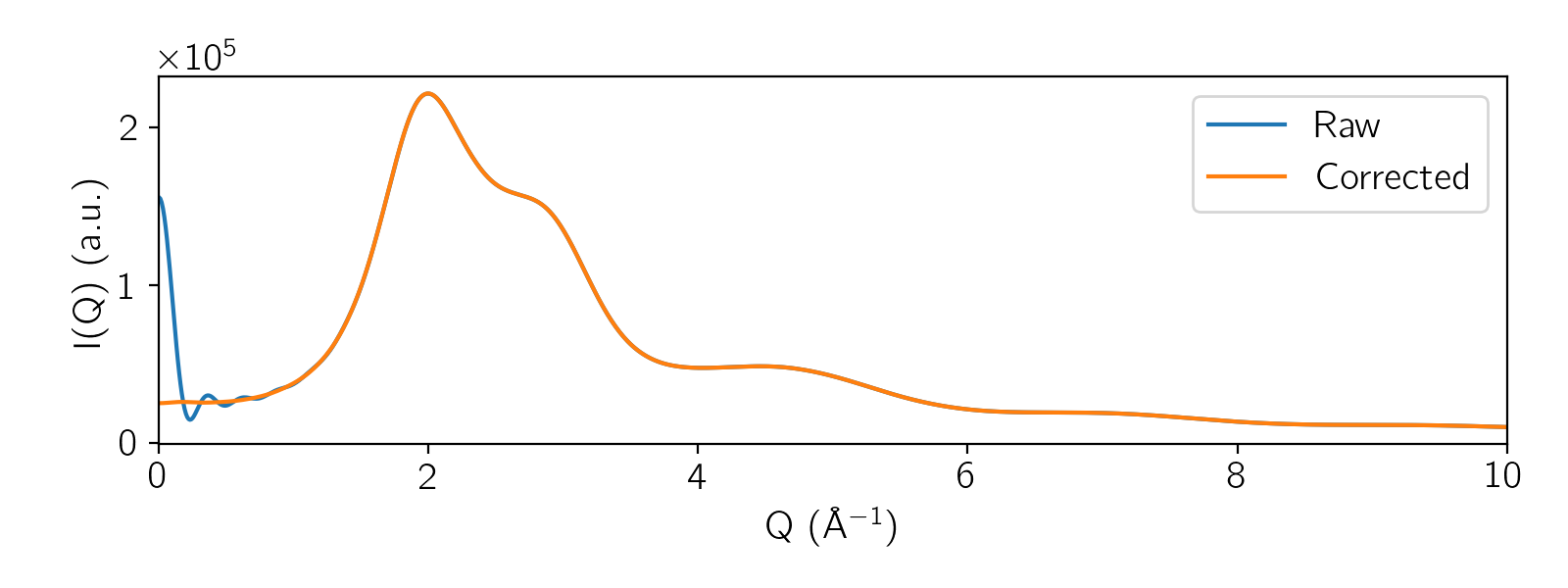
Example: X-ray Scattering of Water:
from grsq.grsq import rdfset_from_dir

V = 122900.85207774633  # volume of MD box
stoich = {'H_v': 8190, 'O_v': 4095}  # number of atoms in MD box
# Helper function to create RDFSet
rdfs = rdfset_from_dir('tests/data/xray_water/',
                       volume=V, stoich=stoich)

qvec = np.arange(0, 10, 0.05)  # create q vector
ig_u = rdfs.get_iq(qvec)  # Calculate scattering
rdfs.vdv_correct()  # apply finite-size corrections
ig_c = rdfs.get_iq(qvec)  # Calculate scattering again

fig, ax = plt.subplots(1, 1, figsize=(9, 5))
ax.plot(qvec, ig_u, label='Raw')
ax.plot(qvec, ig_c, label='Corrected')
ax.set_xlim([0, 10])
ax.set_xlabel('Q (Å$^{-1})$')
ax.set_ylabel('I(Q)')
ax.legend(loc='best');
fig.tight_layout()
Installation
The package is available from PyPi:
pip install grsq
Or clone this repository and add it to your $PYTHONPATH.
Introduction
For each pairwise RDF you have sampled from your system, you should create an RDF object, in this example between the Oxygens and Hydrogens of the solvent-region:
dat = np.genfromtxt('some_data_file.dat')  # has (r,g(r)) as columns in this example
rdf = RDF(dat[:, 0], dat[:, 1],   # r and g(r)
          'O', 'H',   # atom types
          'solvent', 'solvent',  # atom type regions
          n1=4095, n2=8190,  # number of atoms of each type
          volume=122900.85,  # volume in Å of simulation cell
          qvec=qvec)
There are 2 possible regions for your atom types to exist in: 'solute' and 'solvent'.
From a single RDF object, you can calculate the structure factor:
rdf.structure_factor()
as well as the first (atomic), and 2nd term of the x-ray scattering signal:
rdf.term1() + rdf.term2()
You most likely have a large amount of pairwise RDFs from a system of a solute comprised of various elements in a solvent. To make things simple, we can put them all into an RDFSet instance. How to do so most easily depends on how you store your RDF data, naming, data format, etc...
If you follow the naming convention in the documentation of the helper function rdfset_from_dir, this function can help you do so, as in the water example above.
The RDFSet Class
An OrderedDict of RDF objects, which you have to create yourself, you might e.g. already have created a list_of_rdf_objects:
from grsq.grsq import RDFSet
rdfs = RDFSet()
for rdf in list_of_rdf_objects:
    rdfs.add_rdf(rdf)
Or have a look at:
from grsq.grsq import rdfset_from_dir
?rdfset_from_dir
Having an RDFSet is very convenient, as you get access to a bunch of methods:
rdfs.show(): Returns information of the setrdfs.get_iq(qvec=None, cross=False, damping=None)Get the total coherent x-ray scattering signal from entire set. You can specifyqvecandDampingto overwrite whatever is already contained in each RDF object.rdfs.get_solute(): Returns the scattering of only the solute-solute atom type RDFsrdfs.get_solvent(): Returns the scattering of only the solvent-solvent atom type RDFsrdfs.get_cross(): Returns the scattering of only the solute-solvent and solvent-solute atom type RDFsrdfs.get_dv(): Returns the excluded volume-scattering
All methods take qvec and damping as arguments. To use fourier damping functions, parse a damping object to the method:
from grsq.damping import Damping
damping = Damping('lorch', L=r_max)
rdfs.get_solvent(qvec=qvec, damping=damping)
Finite Size corrections
The following finite size corrections are available (see this work for details):
-
rdf.volume_correct(Rl): Apply the volume correction to the RDF, using a spherical $V_l$ volume of radiusRl: $$ g_{lm}^\mathrm{\infty}(r) = \frac{\rho_m}{\rho_\mathrm{eff}} g_{lm}^N(r) = g_{lm}^N(r)\rho_m \frac{V_\mathrm{cell} - V_l}{N_m - \delta_{lm}}, $$ -
rdf.perera_correct(Rl, r_avg): Apply the correction from Perera et al. $$ g^\mathrm{\infty}{lm}(r) = g^N{lm}(r) \left [ 1 + \frac{1 - g^{N,0}}{2} \left( 1 + \tanh \left( \frac{r - \kappa_{lm}}{\alpha_{lm}} \right) \right) \right ]. $$ Where $g^{N,0}$ is obtained by settingr_avgto get the average value of g(r > r_avg), andRl= $\kappa_{lm} / 2$, to be consistent with the volume correction, as well as the recommendations from the original paper. -
rdf.vdv_correct(): Apply the Ganguly / van der Vegt correction: $$ g^\mathrm{\infty}\mathrm{lm}(r) = g^N\mathrm{lm}(r) \frac{N_m}{N_m - \left[ (\Delta N(r) + \delta_{lm}) \left( 1 - \frac{(4/3) \pi r^3}{V_\mathrm{cell}} \right)^{-1} \right]} $$
Support methods:
rdf.fit(Rl_guess, fit_start=25, fit_stop=50): Fit the excluded volume radius.
Can be used together withrdf.volume_correct(Rl)to estimateRl. It minimizes g(r) - 1 fromfit_starttofit_stop
Try ?RDF or help(RDF) for more info.
The RDFSet also has the method rdfs.vdv_correct() that apply the van der Vegt correction to all relevant RDFs automatically.
Release history Release notifications | RSS feed


Download files
Download the file for your platform. If you're not sure which to choose, learn more about installing packages.
Source Distribution
Built Distribution
Filter files by name, interpreter, ABI, and platform.
If you're not sure about the file name format, learn more about wheel file names.
Copy a direct link to the current filters
File details
Details for the file grsq-1.3.1.tar.gz.
File metadata
- Download URL: grsq-1.3.1.tar.gz
- Upload date:
- Size: 27.0 kB
- Tags: Source
- Uploaded using Trusted Publishing? No
- Uploaded via: twine/6.1.0 CPython/3.11.11
File hashes
| Algorithm | Hash digest | |
|---|---|---|
| SHA256 |
b4d4bca3940804dc35a2307b602dd757300374884d2e3eb7ee4e003799fd41b7
|
|
| MD5 |
d25a7d3d0639516b15c811cb800d5e33
|
|
| BLAKE2b-256 |
c6022c442c63f7f10d80b9ab7860d060e3a79ed5076a8c7bb91871ee70f9b363
|
File details
Details for the file grsq-1.3.1-py3-none-any.whl.
File metadata
- Download URL: grsq-1.3.1-py3-none-any.whl
- Upload date:
- Size: 21.3 kB
- Tags: Python 3
- Uploaded using Trusted Publishing? No
- Uploaded via: twine/6.1.0 CPython/3.11.11
File hashes
| Algorithm | Hash digest | |
|---|---|---|
| SHA256 |
93e6a244fd5dfa19d3a6386a1549bced61f7ab0d8a09f1fb10ee3ffdd05a36ae
|
|
| MD5 |
c79e60c941459ecad0de2a71d270ecfc
|
|
| BLAKE2b-256 |
9254fc75c84be94378b67f82deba529f1041ed1f6e7b05099d9694a40b877be3
|


