
ipyspeck
A Jupyter Widget for rendering beautiful molecular structures using Speck.
| Latest Release |

|
| PyPI Downloads |


|
About
Speck is a molecule renderer with the goal of producing figures that are as attractive as they are practical. Express your molecule clearly and with style.
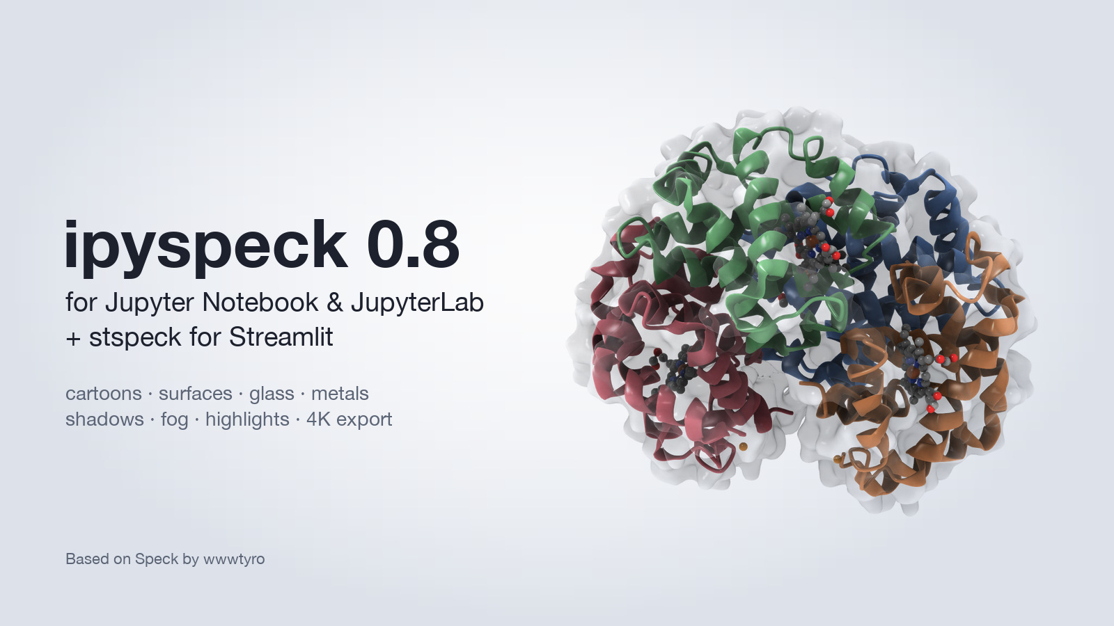
ipyspeck brings Speck to Jupyter Notebook and JupyterLab: ambient-occlusion rendering of atoms and bonds, protein and nucleic-acid cartoons, molecular surfaces (optionally transparent), metallic and glossy materials, shadows, depth fog, highlighting, trajectories, unit cells and high-resolution image and animation export. The same viewer is available for Streamlit as stspeck.
Version Compatibility
⚠️ IMPORTANT: Version Compatibility Notice
ipyspeck 0.8.x requires:
- Jupyter Notebook 6 or JupyterLab 3 / 4
- ipywidgets 7 or 8
- Python >= 3.8
For older environments, use ipyspeck 0.6.x:
- JupyterLab 2.x → use
ipyspeck<0.7- ipywidgets < 7.0 → use
ipyspeck<0.7- Python < 3.8 → use
ipyspeck<0.7Migration Notes:
- Version 0.8.0 works with Classic Notebook 6 and JupyterLab 3 and 4, on ipywidgets 7 and 8
- Version 0.7.0+ uses the modern JupyterLab 3+ federated extension system
- Version 0.7.0+ supports both ipywidgets 7.x and 8.x with backward compatibility
- Version 0.7.0+ uses Lumino (LuminoJS) instead of deprecated PhosphorJS
Installation
Standard Installation
For JupyterLab 3+ and ipywidgets 7+:
pip install ipyspeck
That's it! The extension will be automatically enabled in JupyterLab 3+.
Legacy Installation (JupyterLab 2.x)
For older JupyterLab versions:
pip install "ipyspeck<0.7"
jupyter nbextension enable --py --sys-prefix ipyspeck
jupyter labextension install ipyspeck
Development Installation
For developers who want to contribute:
git clone https://github.com/denphi/speck.git
cd speck/jupyter
npm install && npm run build
pip install -e .
Usage
Quick start
from ipyspeck import Speck

Speck.from_pdb_id("4HHB")                  # RCSB entry (mmCIF), shown as a cartoon
Speck.from_alphafold("Q8W3K0")             # AlphaFold model, colored by confidence
Speck.from_file("ligand.sdf")              # PDB, mmCIF, SDF / MOL or XYZ, also .gz
Every setting below is a constructor argument and can also be changed live
(w.surface = True). The toolbar in the top right switches styles and looks,
toggles cartoon, surface and ligands, sets standard views, auto-rotates,
focuses by tapping, opens a color menu (cartoon, surface and atom color
schemes) and saves a PNG. Set the size with w.layout.height = "500px".
The viewer works with touch (one finger rotates, two fingers pinch to zoom and pan) and keyboard (Tab to the toolbar or the molecule; arrows rotate, Shift+arrows pan, + / - zoom, 0 recenters, F focuses at the center); toolbar buttons are labelled for screen readers.
Cartoons, surfaces and ligands
w = Speck.from_pdb_id("4HHB", cartoonColor="chain")   # 'ss', 'chain', 'rainbow', 'plddt' or '#rrggbb'
w.surface = True                  # solvent-excluded molecular surface
w.surfaceOpacity = 0.3            # see the cartoon and ligands through it
w.cartoonAtoms = "sidechains"     # also 'ligands' (default), 'all', 'none'
w.ligands = False                 # hide ligands in any view
Looks, lighting and materials
w.apply_preset("cover")           # default, matte, glossy, toon, cover, metal, glass, goodsell
w.shadows = 0.6                   # cast shadows from the key light
w.fog = 0.4                       # depth cue toward fogColor
w.rim = 0.3                       # rim light along silhouettes
w.specular, w.gloss = 0.5, 0.7    # highlights
w.metallic, w.metallicAtoms = 1.0, "metals"   # shiny metals, matte organics
w.outline, w.outlineColor = 0.5, "#2d2466"
w.autoRotate = True               # turntable spin (also a toolbar toggle)
The looks are also in the toolbar's sparkle menu.
Studio floor, illustration style and cutaway
w.floor, w.floorReflection = 0.9, 0.3     # soft contact shadow and reflection (off by default)
w.apply_preset("goodsell")                # Goodsell-style illustration: flat colors per chain
w.atomColor = "type"                      # atoms by chain, entity, type (protein / RNA), ss, rainbow
w.palette = "colorblind"                  # goodsell, pastel, colorblind, viridis, grays, default
w.cutaway = 0.5                           # slice off the front half to look inside
w.cutawayAxis = "z"                       # plane facing the camera ("view") or fixed across x / y / z
w.cutawayLight = 0.6                      # light entering through the cut, for the inside
The floor works on any background (it only adds shadow and reflection). outlineMode="molecules"
outlines only the edges between molecules, as in illustrations. Cut atoms and surfaces are capped,
so capsids and ribosomes open up like a cross-section; a fixed axis keeps the cut in place on the
molecule while you rotate it.
Element colors
w.colorScheme = "jmol"                                  # speck, jmol, rasmol, newcpk
w.atomColors = {"Au": "#ffcc33", "S": [0.9, 0.8, 0.2]}  # per element, on top of the palette
Both are regular settings: they can be passed to the constructor, work before the viewer is
displayed, and the toolbar's color menu updates colorScheme.
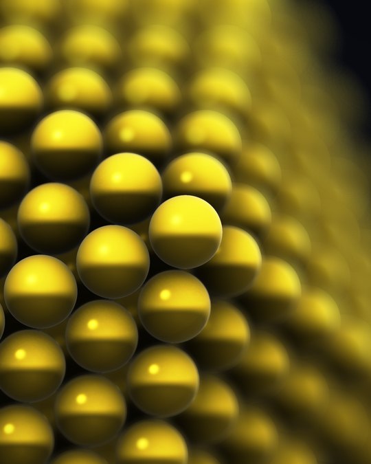
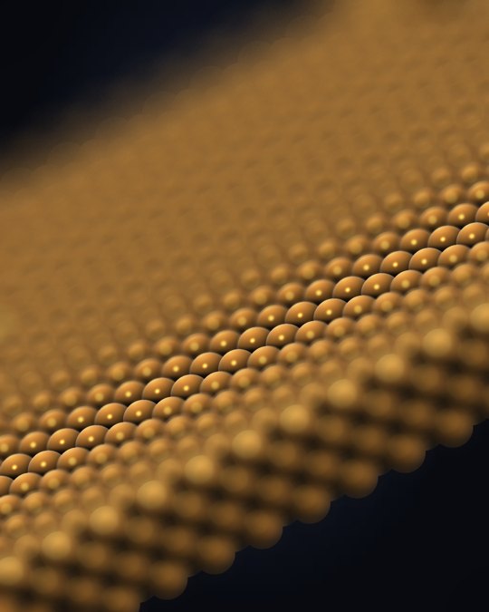
Macro look (depth of field)
Blur grows with the distance to the focal plane and with zoom, like a macro lens:
zoom in on a detail and keep it sharp with dofFocus.
w = Speck.from_pdb_id("4HHB", cartoon=True, highlight={"resName": "HEM", "chain": "A"})
w.dofFocus = {"resName": "HEM", "chain": "A"}   # stays in focus as you rotate
w.dofStrength = 1.2                              # 1 - 2 for a macro look (max 3)
Or tap to focus: turn on the focus button in the toolbar (or hold Alt / Option) and click the
point that should be sharp. The depth under the cursor becomes dofPosition (depth of field
switches on if it was off), and the value is synced back to Python.
The aperture button next to it switches depth of field off and on (dofStrength).
Highlighting
w.highlight = {"resName": "HEM"}   # keys: index, chain, resName, resSeq, name, element, ligands
w.highlight = {"chain": "A", "resSeq": ["40-60"]}
w.highlightScale = 1.3
w.ghost = 0.6                      # fade everything else
Figures and animations
w.save_image("figure.png", width=3000)                 # supersampled PNG, up to 4096 px
w.save_animation("turn.gif", frames=60)                # turntable; .mp4 needs imageio
w.save_animation("traj.mp4", mode="trajectory")        # every frame of the data
saved = w.camera                                       # ...later: w.camera = saved
Exports render in the browser after the cell finishes; the file appears a moment later.
Videos
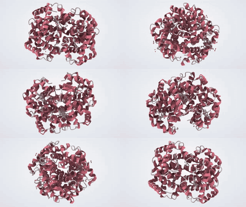
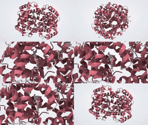
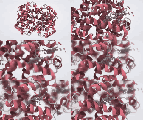
One line makes a video; the viewer shows its progress, and the file appears next to the notebook:
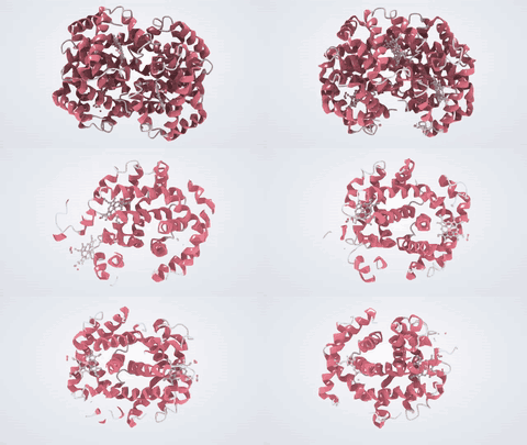
w = Speck.from_pdb_id("4HHB", cartoon=True)
w.preview("tour")                                          # watch it first, in the widget
w.save_video("hemoglobin.mp4", "tour", title="Hemoglobin")
 spin |
 tour |
 focus |
 reveal |
Ready-made videos: spin, rock, orbit, tour and focus (visit the largest ligand, or
target={"chain": "B"}), reveal (cut open), trajectory (NMR ensembles, MD) and showcase.
Options: seconds=, title= / subtitle=, size= ("1080p", "4k", "square", "vertical"
for phones), quality="draft" for a quick test, background=["#1b2330", "#07090d"]. Without
code, the viewer's clapperboard button offers the same videos and a Save video button.
Step-by-step notebooks, from a first video to your own storyboard: example/videos.
A guided tour
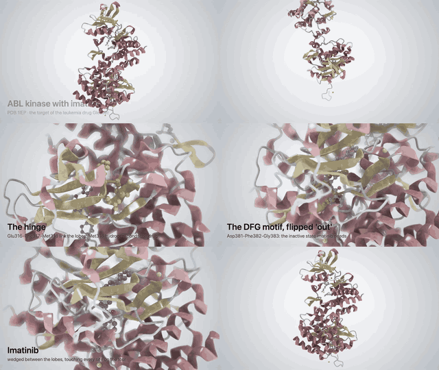
A one-minute tour of ABL kinase with imatinib (PDB 1IEP), built from a list of stops with
shots.visit, which flies to a site, colors it, shows its side chains, captions it and focuses on it:
stops = [("The hinge", {"chain": "A", "resSeq": [316, 317, 318]}, "Met318 hydrogen-bonds the drug"),
         ("The gatekeeper, Thr315", {"chain": "A", "resSeq": 315}, "T315I causes drug resistance"),
         ("The DFG motif", {"chain": "A", "resSeq": [381, 382, 383]}, "flipped 'out' for the drug")]
film = [shots.visit(site, 6, title=name, subtitle=why, color="#ff9f1c") for name, site, why in stops]
w.save_video("tour.mp4", film)
The full film is in example/videos/07_guided_tour.ipynb.
For your own moves, put shots together:
from ipyspeck import shots

heme = {"resName": "HEM", "chain": "A"}
film = [
    shots.together(shots.orbit(6, degrees=180), shots.title("Hemoglobin")),
    shots.crossfade(2, surface=True, surfaceOpacity=0.35),
    shots.fly_to(heme, 3, face=True),
    shots.rack_focus(heme, 2),
    shots.home(3),
]
w.save_video("hemoglobin_story.mp4", film)
Every frame is fully shaded, with ambient occlusion fixed to the molecule, so videos do not
flicker. MP4s are made in the browser (Chrome, Edge, Safari 16.4+, Firefox 130+); .gif,
.webm, .mov or a folder of PNGs are written in Python: pip install "ipyspeck[video]" adds
what they need (Pillow, and imageio with ffmpeg).
Structures from Python
Speck.from_file("structure.cif")   # .pdb/.ent, .cif/.mmcif, .sdf/.mol, .xyz/.extxyz, optionally .gz
Speck.from_pdb_id("4V6X")           # a ribosome: 237,685 atoms, only available as mmCIF
Speck.from_pdb_id("1STM", assembly=1)   # biological assembly: the whole 60-copy virus capsid
Speck.from_mdtraj(mdtraj.load("run.xtc", top="system.gro"), stride=10)   # MD trajectory
Speck.from_mdanalysis(u.select_atoms("protein"), step=10)                # MDAnalysis Universe / AtomGroup
Speck.from_ase(atoms)              # ase.Atoms or a list (trajectory); periodic cells shown
Speck.from_rdkit(mol)              # needs 3D coordinates (AllChem.EmbedMolecule); keeps its bonds
Speck.from_pymatgen(structure)     # Structure (with its cell) or Molecule
The format is detected from the text, so Speck(data=...) accepts any of them. mmCIF, the
PDB's standard format, covers entries that PDB files cannot hold (over 99,999 atoms or 62
chains, multi-character chain IDs, five-character ligand codes); from_pdb_id downloads it
by default (format="pdb" for the legacy file). Bonds listed in the file (PDB CONECT,
mmCIF _struct_conn, SDF / MOL bond tables) are always drawn, including long metal bonds.
Multi-frame XYZ, multi-model PDB or mmCIF and multi-conformer SDF data are trajectories: set
w.frame, or display w.trajectory_controls() for a play button and slider. MD trajectories
(from_mdtraj, from_mdanalysis, or w.set_trajectory(coords) with an array of shape
(frames, atoms, 3) in Å) keep residues and chains, so cartoons follow the motion; their frames
travel to the browser as binary coordinates rather than repeated text.
Large structures stay interactive: ribosomes and capsids (200k+ atoms) load in the background, render as atoms, cartoons or surfaces at full frame rate, and structure data reaches the browser gzipped.
If Jupyter serves an older copy of the browser extension than the installed package (for
example one left in ~/.local/share/jupyter by an earlier pip install --user), ipyspeck
warns with the folder to remove; restart Jupyter afterwards.
See example/showcase.ipynb for a tour of every feature.
Streamlit
The same viewer and settings are available for Streamlit apps in the separate stspeck package:
pip install stspeck
import stspeck
stspeck.speck(**stspeck.fetch_alphafold("Q8W3K0"), preset="cover", height=500)
Features
- 🎨 Publication-quality rendering: ambient occlusion, shadows, fog, rim light, outlines
- 🧬 Protein and nucleic-acid cartoons with computed or file secondary structure
- 🫧 Molecular surfaces, optionally transparent, colored by element, chain, residue or pLDDT
- ✨ Glossy and metallic materials, with metal-only reflections for nanoparticles and crystals
- 🔦 Highlighting and ghosting of any atom selection
- 🎞️ Trajectories, unit cells, and high-resolution image, GIF and MP4 export
- 🧪 Loaders for RCSB, AlphaFold DB, ASE, RDKit and pymatgen
- 🔌 Jupyter Notebook 6, JupyterLab 3 and 4, ipywidgets 7 and 8; Streamlit via stspeck
Gallery
Rendered with ipyspeck (see example/showcase.ipynb for the settings behind these looks). Click an image to open the notebook that reproduces it (same settings and camera), or see them all in example/gallery.
Macro photography (depth of field)
 Gold nanoparticle, 923 atoms |
 Copper surface |
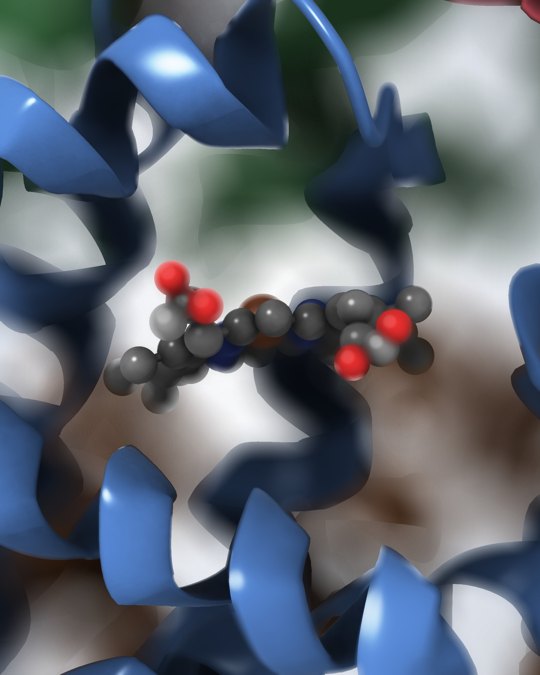 Heme in hemoglobin (4HHB) |
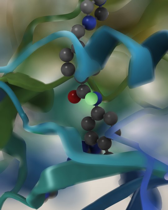 Imatinib in ABL kinase (1IEP) |
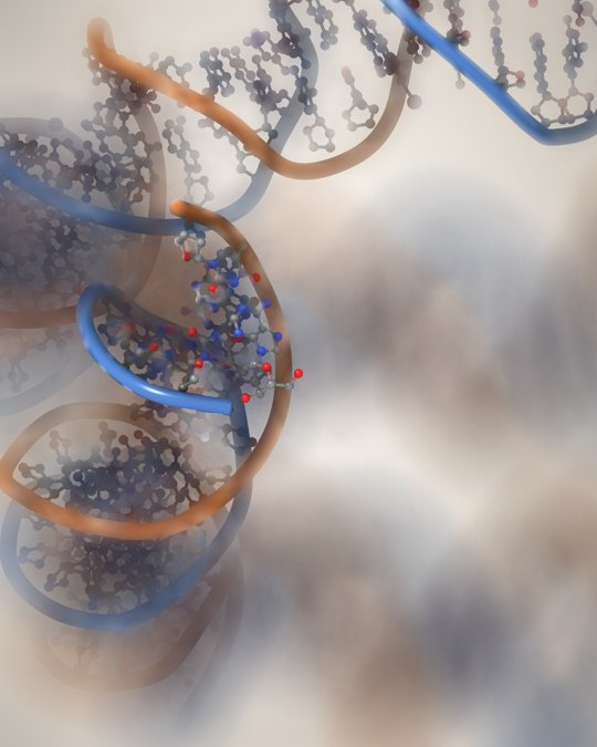 Nucleosome DNA (1KX5) |
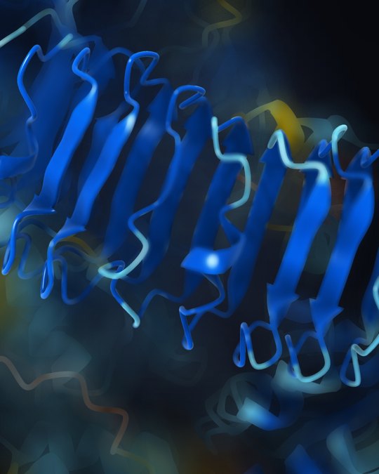 AlphaFold RPP7 repeat domain |
Proteins and complexes
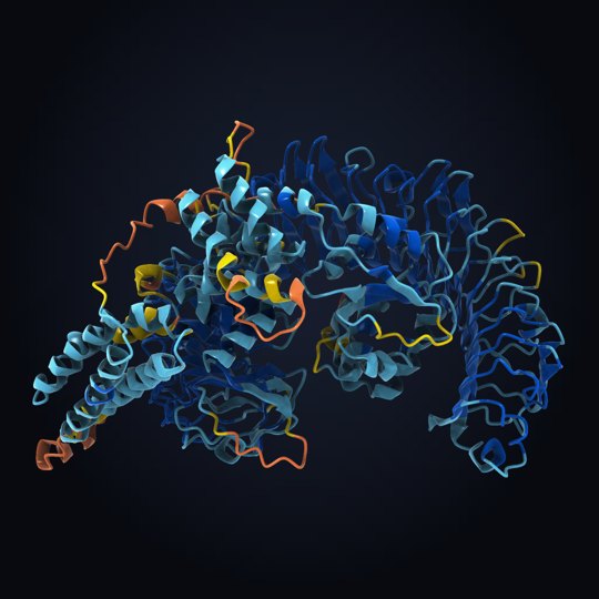 AlphaFold RPP7, by pLDDT |
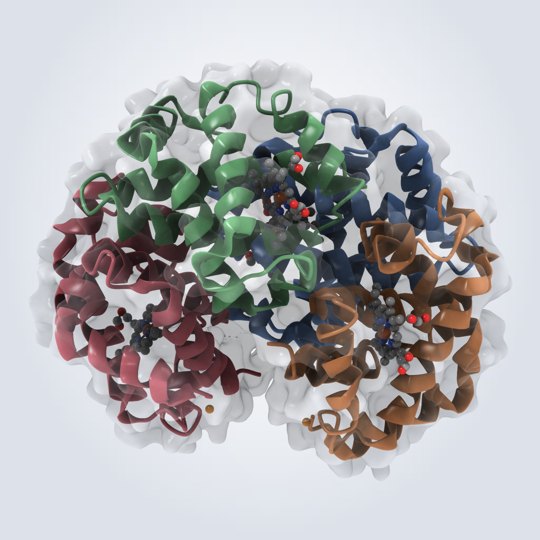 Hemoglobin, glass surface (4HHB) |
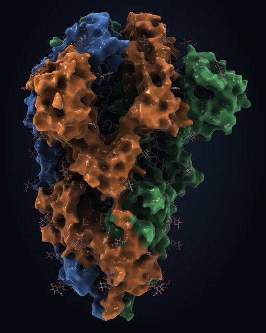 SARS-CoV-2 spike (6VXX) |
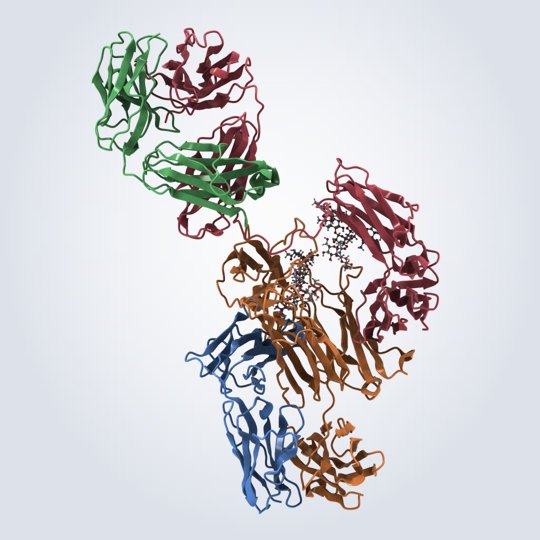 IgG antibody (1IGT) |
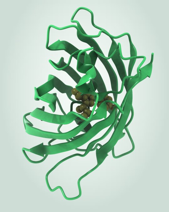 Green fluorescent protein (1EMA) |
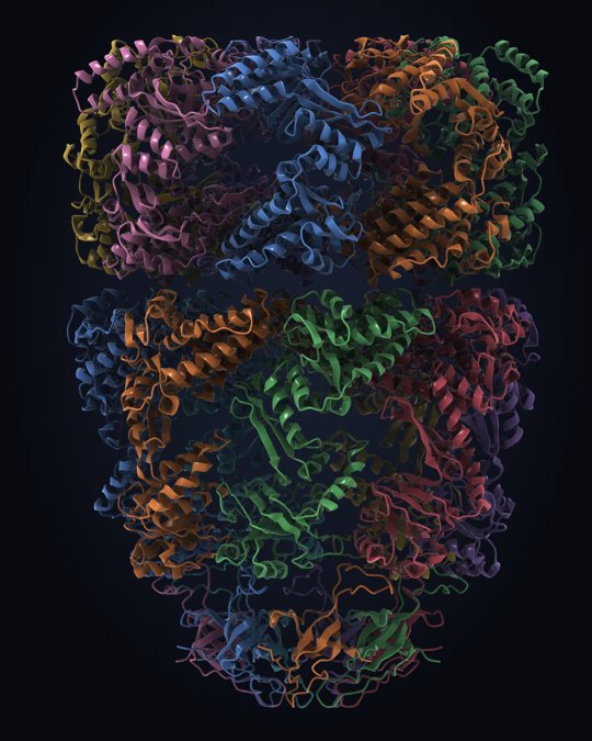 GroEL–GroES chaperonin (1AON) |
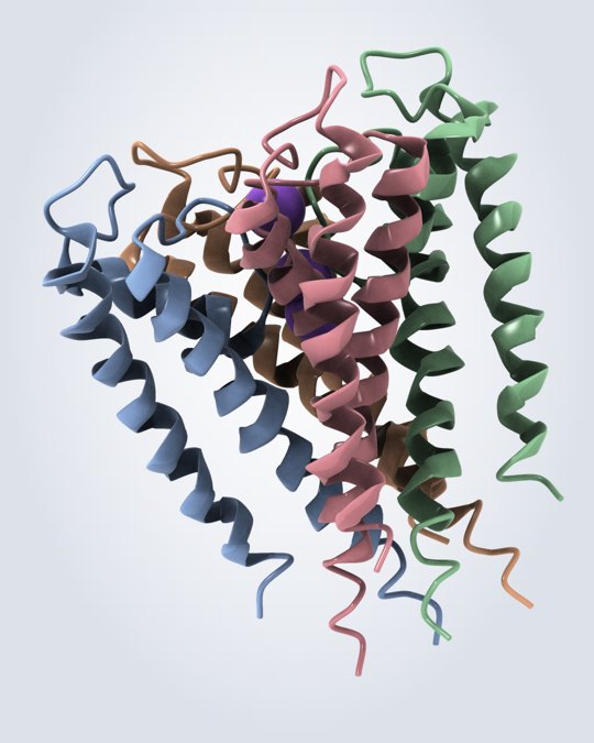 KcsA K⁺ channel (1BL8) |
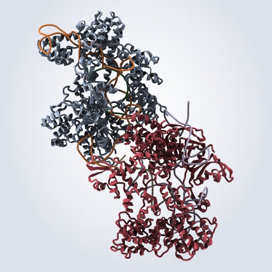 CRISPR-Cas9 with guide RNA (4OO8) |
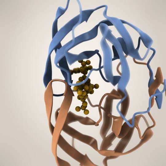 HIV protease + saquinavir (1HXB) |
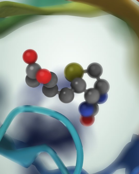 Streptavidin–biotin (1STP) |
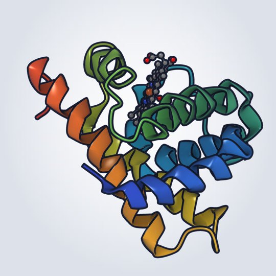 Myoglobin, toon style (1MBN) |
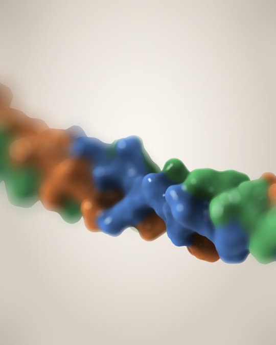 Collagen triple helix (1BKV) |
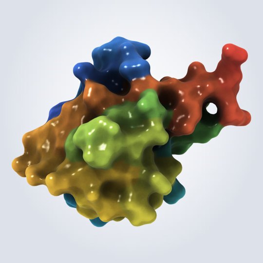 Ubiquitin surface (1UBQ) |
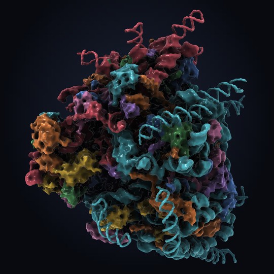 Human 80S ribosome, 237,685 atoms (4V6X) |
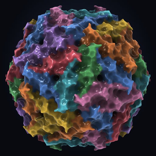 Virus capsid, all 60 copies (1STM) |
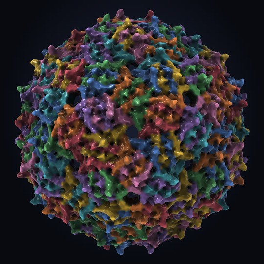 Bacteriophage MS2 capsid, 180 copies (2MS2) |
Nucleic acids
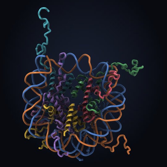 Nucleosome (1KX5) |
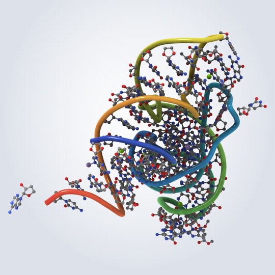 Transfer RNA (1EHZ) |
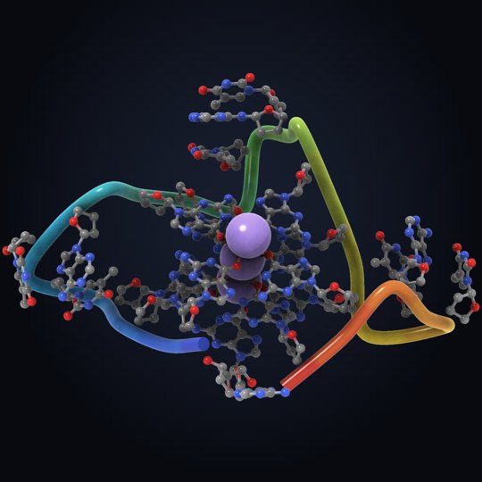 G-quadruplex with K⁺ (1KF1) |
Studio floor, illustration and cutaway
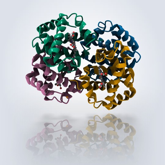 Hemoglobin on the studio floor (4HHB) |
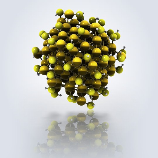 Gold–thiolate cluster on the studio floor |
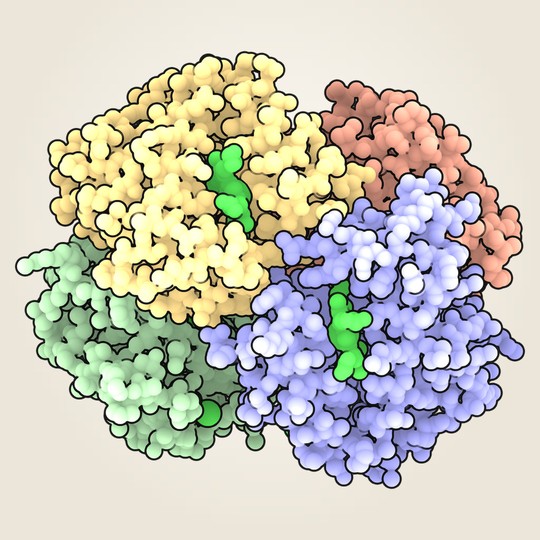 Hemoglobin, Goodsell style (4HHB) |
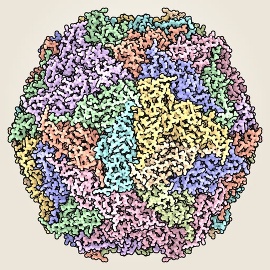 Virus capsid, Goodsell style (1STM) |
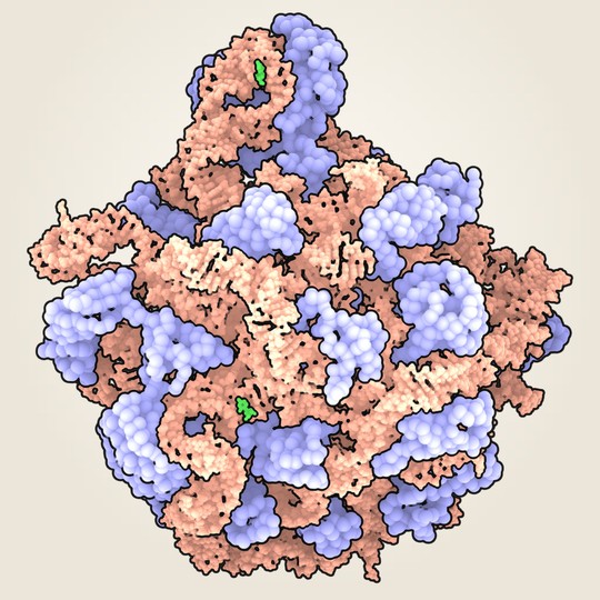 Ribosome large subunit, Goodsell style (1FFK) |
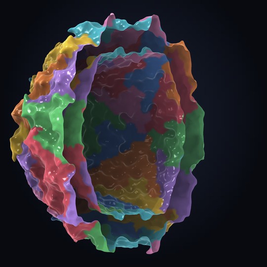 Virus capsid, cut open (1STM) |
Chemistry and materials
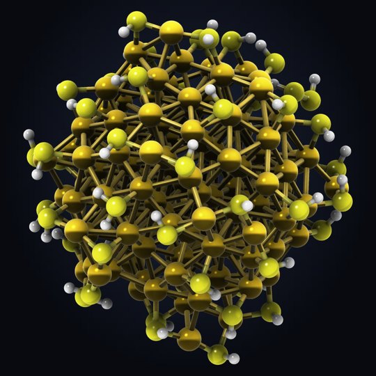 Gold–thiolate cluster |
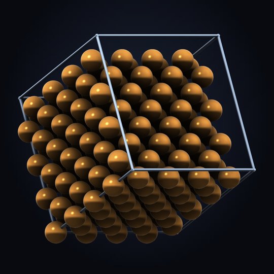 Copper crystal and unit cell |
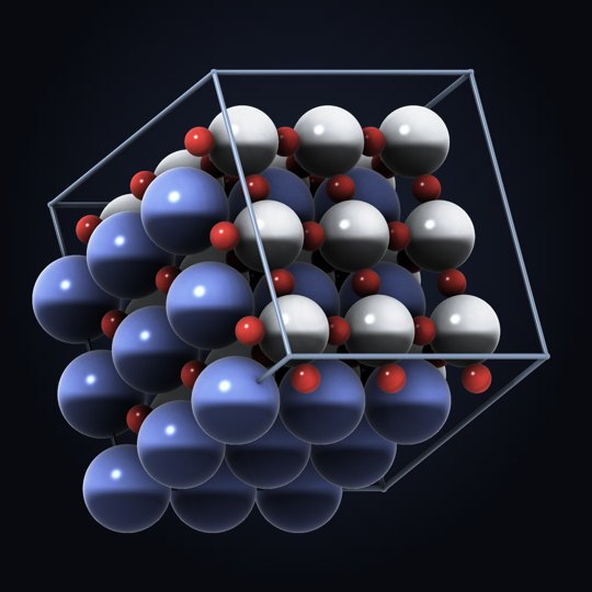 SrTiO₃ perovskite |
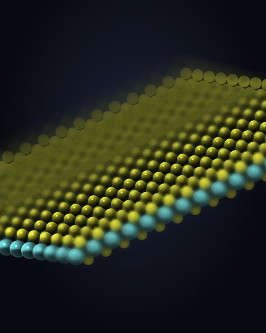 MoS₂ monolayer |
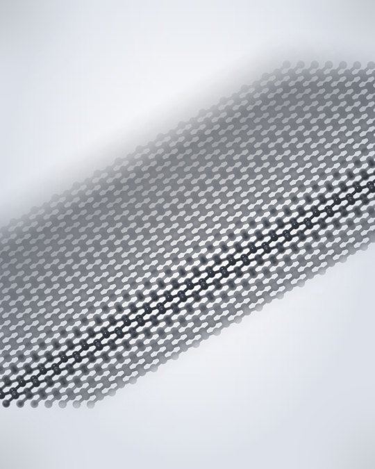 Graphene |
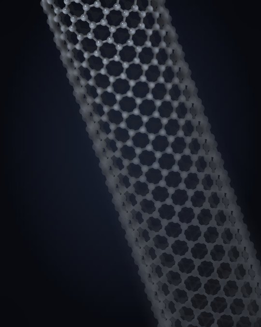 Carbon nanotube |
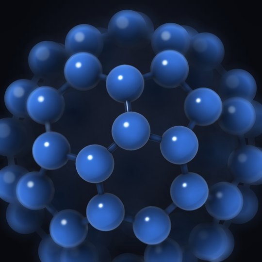 C₆₀ buckminsterfullerene |
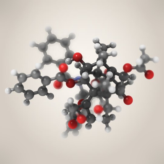 Taxol (paclitaxel) |
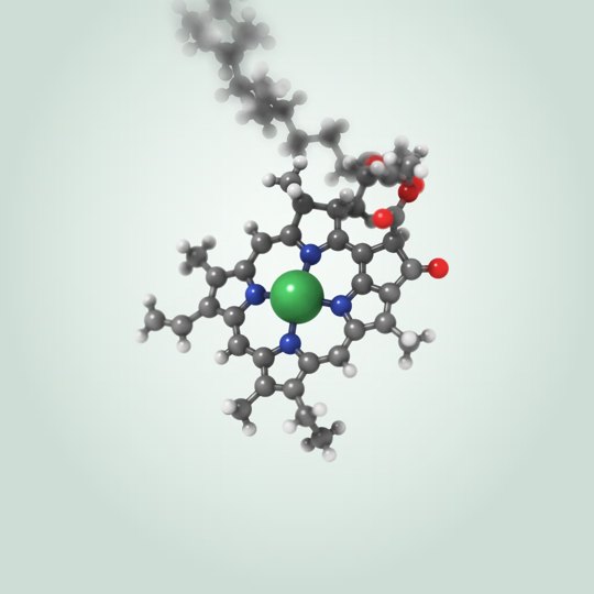 Chlorophyll a |
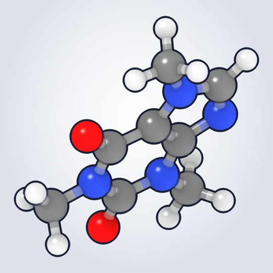 Caffeine |
Development
The widget lives in jupyter/; the renderer and viewer it shares with stspeck live in
core/ and are built first.
cd jupyter
npm install
npm run build          # core, TypeScript, notebook and lab extensions (dev)
npm run build:prod     # production build
npm test               # model unit tests
pip install -e .
License
BSD-3-Clause (see LICENSE). ipyspeck is based on Speck by wwwtyro,
which is in the public domain (see LICENSE-SPECK).
Author
Daniel Mejia (Denphi) - denphi@denphi.com
Links
1 maintainer

Release files for ipyspeck 0.8.4
For a detailed explanation of source distributions (sdists) and built distributions (wheels), please see the package formats documentation.
Source distribution (sdist)
| File | Size | Uploaded | |
|---|---|---|---|
| ipyspeck-0.8.4.tar.gz | 641.5 kB | Details |
Built distribution (wheel)
| File | Interpreter | ABI | Platform | Reset |
|---|---|---|---|---|
| ipyspeck-0.8.4-py3-none-any.whl | Python 3 | none | any | Details |
Total release size: 1.6 MB
Release files / ipyspeck-0.8.4.tar.gz
| Download URL | ipyspeck-0.8.4.tar.gz |
|---|---|
| Size | 641.5 kB |
| Tags | Source |
|
SHA-256 checksum How to use checksums |
eb39005f2581f74120a7ac1b0e52c1b3e0ad1e30d2ad682bf896a8604494a8d1
|
|
BLAKE2b-256 checksum How to use checksums |
20fdb4a7bec6934d2d4b0ea3918eac6c2e51e1c33b08882f9add3434321505ef
|
| Upload date | |
|
Uploaded using Trusted Publishing? What is trusted publishing? |
No |
| Uploaded via |
twine/7.0.0 CPython/3.12.13
|
Release files / ipyspeck-0.8.4-py3-none-any.whl
| Download URL | ipyspeck-0.8.4-py3-none-any.whl |
|---|---|
| Size | 949.6 kB |
| Tags | Python 3 |
|
SHA-256 checksum How to use checksums |
e9510d5ac720e477fb9277a1062f17fd6920bf113b63a0c2b7492503dd6c094a
|
|
BLAKE2b-256 checksum How to use checksums |
45a164ec7a2112625316ff802407e2904f6abda220e383a22c8531621b7e17da
|
| Upload date | |
|
Uploaded using Trusted Publishing? What is trusted publishing? |
No |
| Uploaded via |
twine/7.0.0 CPython/3.12.13
|














