Easy benchmarking of machine learning models with sklearn interface with statistical tests built-in.

Project description
Easy benchmarking of machine learning models with sklearn interface with statistical tests built-in.
Usage for classification problems
First, we consider the plot_classifier_comparison.py demo file. This extends the standard sklearn classifier comparison but also demos the ease of mlpaper to create a performance report.
In this demo, we use the example of the three toy data sets and ten classifiers from the sklearn example:
The mlpaper package can benchmark all of the of these methods and created a properly formatted LaTeX table (with error bars) in a few commands. This generates a results table for copy-and-paste into a ML paper .tex file in a few commands.
Pandas tables with the performance results of all the methods can be built by:
import mlpaper.classification as btc
from mlpaper.classification import STD_BINARY_CURVES, STD_CLASS_LOSS

performance_df, performance_curves_dict = btc.just_benchmark(
    X_train,
    y_train,
    X_test,
    y_test,
    2,
    classifiers,
    STD_CLASS_LOSS,
    STD_BINARY_CURVES,
    ref_method,
)
This benchmarks all the models in classifiers on the data (X_train, y_train, X_test, y_test) for 2-class classification. It uses the loss function described in the dictionaries STD_CLASS_LOSS, and the curves (e.g., ROC, PR) in STD_BINARY_CURVES. The ref_method defines the model that is the reference to compare against for assessing statistically significant performance gains.
The sciprint module formats these tables for scientific presentation. The performance dictionaries can be converted to cleanly formatted tables: correct significant figures, shifting of exponent for compactness, thresholding huge/small (crap limit) results, and correct alignment of decimal points, units in headers, etc. Here we use:
import mlpaper.sciprint as sp

print(
    sp.just_format_it(
        performance_df,
        shift_mod=3,
        unit_dict={"NLL": "nats"},
        crap_limit_min={"AUPRG": -1},
        EB_limit={"AUPRG": -1},
        non_finite_fmt={sp.NAN_STR: "N/A"},
        use_tex=False,
    )
)
to export the results in plain text, or for LaTeX we use:
import mlpaper.sciprint as sp

print(
    sp.just_format_it(
        performance_df,
        shift_mod=3,
        unit_dict={"NLL": "nats"},
        crap_limit_min={"AUPRG": -1},
        EB_limit={"AUPRG": -1},
        non_finite_fmt={sp.NAN_STR: "{--}"},
        use_tex=True,
    )
)
Output
Dataset 0 (Moons)
                          AP        p        AUC        p    AUPRG        p      Brier        p NLL (nats)        p     sphere        p   zero one        p
AdaBoost           0.93(16)   <0.0001  0.950(96)  <0.0001  0.90464  <0.0001  0.42(14)   <0.0001  0.368(80)  <0.0001  0.36(15)   <0.0001  0.075(86)  <0.0001
Decision Tree      0.95(13)   <0.0001  0.966(70)  <0.0001  0.93860  <0.0001  0.18(25)   <0.0001  0.40(71)    0.4072  0.16(22)   <0.0001  0.050(71)  <0.0001
Gaussian Process   0.90(22)   <0.0001  0.95(12)   <0.0001  0.92081  <0.0001  0.27(17)   <0.0001  0.27(11)   <0.0001  0.22(16)   <0.0001  0.025(51)  <0.0001
Linear SVM         0.952(99)  <0.0001  0.950(77)  <0.0001  0.88705  <0.0001  0.34(24)   <0.0001  0.29(16)   <0.0001  0.31(24)   <0.0001  0.15(12)    0.0006
Naive Bayes        0.957(97)  <0.0001  0.957(68)  <0.0001  0.89782  <0.0001  0.34(25)   <0.0001  0.28(18)   <0.0001  0.31(24)   <0.0001  0.13(11)    0.0002
Nearest Neighbors  0.94(14)   <0.0001  0.969(69)  <0.0001  0.93498  <0.0001  0.18(21)   <0.0001  0.42(70)    0.4241  0.15(18)   <0.0001  0.025(51)  <0.0001
Neural Net         0.957(91)  <0.0001  0.957(69)  <0.0001  0.89782  <0.0001  0.33(23)   <0.0001  0.28(15)   <0.0001  0.30(22)   <0.0001  0.100(98)  <0.0001
QDA                0.951(91)  <0.0001  0.950(80)  <0.0001  0.88517  <0.0001  0.34(27)   <0.0001  0.29(21)    0.0003  0.31(25)   <0.0001  0.15(12)    0.0006
RBF SVM            0.93(18)   <0.0001  0.957(94)  <0.0001  0.92081  <0.0001  0.14(20)   <0.0001  0.18(18)   <0.0001  0.12(17)   <0.0001  0.025(51)  <0.0001
Random Forest      0.965(82)  <0.0001  0.949(84)  <0.0001  0.92147  <0.0001  0.31(26)   <0.0001  0.52(70)    0.6099  0.28(24)   <0.0001  0.100(98)  <0.0001
iid                0.53(16)       N/A  0.5(0)         N/A  0(0)         N/A  1.004(22)      N/A  0.695(11)      N/A  1.005(27)      N/A  0.53(17)       N/A
Dataset 0 (Moons) in LaTeX
\begin{tabular}{|l|Sr|Sr|Sr|Sr|Sr|Sr|Sr|}
\toprule
{}                &       {AP} &      {p} &      {AUC} &      {p} &  {AUPRG} &      {p} &    {Brier} &      {p} & {NLL (nats)} &      {p} &   {sphere} &      {p} & {zero one} &      {p} \\
\midrule
AdaBoost          &  0.93(16)  &  <0.0001 &  0.950(96) &  <0.0001 &  0.90464 &  <0.0001 &  0.42(14)  &  <0.0001 &    0.368(80) &  <0.0001 &  0.36(15)  &  <0.0001 &  0.075(86) &  <0.0001 \\
Decision Tree     &  0.95(13)  &  <0.0001 &  0.966(70) &  <0.0001 &  0.93860 &  <0.0001 &  0.18(25)  &  <0.0001 &    0.40(71)  &   0.4072 &  0.16(22)  &  <0.0001 &  0.050(71) &  <0.0001 \\
Gaussian Process  &  0.90(22)  &  <0.0001 &  0.95(12)  &  <0.0001 &  0.92081 &  <0.0001 &  0.27(17)  &  <0.0001 &    0.27(11)  &  <0.0001 &  0.22(16)  &  <0.0001 &  0.025(51) &  <0.0001 \\
Linear SVM        &  0.952(99) &  <0.0001 &  0.950(77) &  <0.0001 &  0.88705 &  <0.0001 &  0.34(24)  &  <0.0001 &    0.29(16)  &  <0.0001 &  0.31(24)  &  <0.0001 &  0.15(12)  &   0.0006 \\
Naive Bayes       &  0.957(97) &  <0.0001 &  0.957(68) &  <0.0001 &  0.89782 &  <0.0001 &  0.34(25)  &  <0.0001 &    0.28(18)  &  <0.0001 &  0.31(24)  &  <0.0001 &  0.13(11)  &   0.0002 \\
Nearest Neighbors &  0.94(14)  &  <0.0001 &  0.969(69) &  <0.0001 &  0.93498 &  <0.0001 &  0.18(21)  &  <0.0001 &    0.42(70)  &   0.4241 &  0.15(18)  &  <0.0001 &  0.025(51) &  <0.0001 \\
Neural Net        &  0.957(91) &  <0.0001 &  0.957(69) &  <0.0001 &  0.89782 &  <0.0001 &  0.33(23)  &  <0.0001 &    0.28(15)  &  <0.0001 &  0.30(22)  &  <0.0001 &  0.100(98) &  <0.0001 \\
QDA               &  0.951(91) &  <0.0001 &  0.950(80) &  <0.0001 &  0.88517 &  <0.0001 &  0.34(27)  &  <0.0001 &    0.29(21)  &   0.0003 &  0.31(25)  &  <0.0001 &  0.15(12)  &   0.0006 \\
RBF SVM           &  0.93(18)  &  <0.0001 &  0.957(94) &  <0.0001 &  0.92081 &  <0.0001 &  0.14(20)  &  <0.0001 &    0.18(18)  &  <0.0001 &  0.12(17)  &  <0.0001 &  0.025(51) &  <0.0001 \\
Random Forest     &  0.965(82) &  <0.0001 &  0.949(84) &  <0.0001 &  0.92147 &  <0.0001 &  0.31(26)  &  <0.0001 &    0.52(70)  &   0.6099 &  0.28(24)  &  <0.0001 &  0.100(98) &  <0.0001 \\
iid               &  0.53(16)  &     {--} &  0.5(0)    &     {--} &  0(0)    &     {--} &  1.004(22) &     {--} &    0.695(11) &     {--} &  1.005(27) &     {--} &  0.53(17)  &     {--} \\
\bottomrule
\end{tabular}
Dataset 1 (Circles)
                           AP        p        AUC        p      AUPRG        p      Brier        p NLL (nats)        p     sphere        p   zero one        p
AdaBoost           0.938(82)   <0.0001  0.89(12)   <0.0001  0.76091    <0.0001  0.773(96)  <0.0001  0.576(50)  <0.0001  0.73(12)   <0.0001  0.17(13)   <0.0001
Decision Tree      0.86(16)    <0.0001  0.80(13)   <0.0001  0.76316    <0.0001  0.80(52)    0.3009  2.8(18)     0.0270  0.68(45)    0.0792  0.20(13)    0.0003
Gaussian Process   0.977(47)   <0.0001  0.964(60)  <0.0001  0.93049    <0.0001  0.39(23)   <0.0001  0.33(14)   <0.0001  0.36(23)   <0.0001  0.100(98)  <0.0001
Linear SVM         0.53(18)     0.1621  0.51(21)    0.8580  0.19756     0.3660  1.066(80)   0.1521  0.726(41)   0.1514  1.079(96)   0.1531  0.60(16)    1.0000
Naive Bayes        0.9983(82)  <0.0001  0.997(13)  <0.0001  0.996(21)  <0.0001  0.64(20)   <0.0001  0.48(12)   <0.0001  0.63(21)   <0.0001  0.30(15)    0.0003
Nearest Neighbors  0.996(15)   <0.0001  0.966(49)  <0.0001  0.991(47)  <0.0001  0.30(16)   <0.0001  0.23(11)   <0.0001  0.28(16)   <0.0001  0.075(86)  <0.0001
Neural Net         0.993(23)   <0.0001  0.990(32)  <0.0001  0.982(79)  <0.0001  0.69(14)   <0.0001  0.525(74)  <0.0001  0.65(16)   <0.0001  0.25(15)   <0.0001
QDA                0.9983(83)  <0.0001  0.997(11)  <0.0001  0.996(32)  <0.0001  0.63(19)   <0.0001  0.47(11)   <0.0001  0.61(20)   <0.0001  0.28(15)   <0.0001
RBF SVM            0.979(44)   <0.0001  0.966(63)  <0.0001  0.93680    <0.0001  0.34(22)   <0.0001  0.29(14)   <0.0001  0.31(22)   <0.0001  0.100(98)  <0.0001
Random Forest      0.90(13)    <0.0001  0.85(16)   <0.0001  0.64512     0.0021  0.65(30)    0.0070  0.48(19)    0.0094  0.62(31)    0.0047  0.23(14)    0.0006
iid                0.60(16)        N/A  0.5(0)         N/A  0(0)           N/A  1.071(85)      N/A  0.729(43)      N/A  1.08(11)       N/A  0.60(16)       N/A
Dataset 1 (Circles) in LaTeX
\begin{tabular}{|l|Sr|Sr|Sr|Sr|Sr|Sr|Sr|}
\toprule
{}                &        {AP} &      {p} &      {AUC} &      {p} &    {AUPRG} &      {p} &    {Brier} &      {p} & {NLL (nats)} &      {p} &   {sphere} &      {p} & {zero one} &      {p} \\
\midrule
AdaBoost          &  0.938(82)  &  <0.0001 &  0.89(12)  &  <0.0001 &  0.76091   &  <0.0001 &  0.773(96) &  <0.0001 &    0.576(50) &  <0.0001 &  0.73(12)  &  <0.0001 &  0.17(13)  &  <0.0001 \\
Decision Tree     &  0.86(16)   &  <0.0001 &  0.80(13)  &  <0.0001 &  0.76316   &  <0.0001 &  0.80(52)  &   0.3009 &    2.8(18)   &   0.0270 &  0.68(45)  &   0.0792 &  0.20(13)  &   0.0003 \\
Gaussian Process  &  0.977(47)  &  <0.0001 &  0.964(60) &  <0.0001 &  0.93049   &  <0.0001 &  0.39(23)  &  <0.0001 &    0.33(14)  &  <0.0001 &  0.36(23)  &  <0.0001 &  0.100(98) &  <0.0001 \\
Linear SVM        &  0.53(18)   &   0.1621 &  0.51(21)  &   0.8580 &  0.19756   &   0.3660 &  1.066(80) &   0.1521 &    0.726(41) &   0.1514 &  1.079(96) &   0.1531 &  0.60(16)  &   1.0000 \\
Naive Bayes       &  0.9983(82) &  <0.0001 &  0.997(13) &  <0.0001 &  0.996(21) &  <0.0001 &  0.64(20)  &  <0.0001 &    0.48(12)  &  <0.0001 &  0.63(21)  &  <0.0001 &  0.30(15)  &   0.0003 \\
Nearest Neighbors &  0.996(15)  &  <0.0001 &  0.966(49) &  <0.0001 &  0.991(47) &  <0.0001 &  0.30(16)  &  <0.0001 &    0.23(11)  &  <0.0001 &  0.28(16)  &  <0.0001 &  0.075(86) &  <0.0001 \\
Neural Net        &  0.993(23)  &  <0.0001 &  0.990(32) &  <0.0001 &  0.982(79) &  <0.0001 &  0.69(14)  &  <0.0001 &    0.525(74) &  <0.0001 &  0.65(16)  &  <0.0001 &  0.25(15)  &  <0.0001 \\
QDA               &  0.9983(83) &  <0.0001 &  0.997(11) &  <0.0001 &  0.996(32) &  <0.0001 &  0.63(19)  &  <0.0001 &    0.47(11)  &  <0.0001 &  0.61(20)  &  <0.0001 &  0.28(15)  &  <0.0001 \\
RBF SVM           &  0.979(44)  &  <0.0001 &  0.966(63) &  <0.0001 &  0.93680   &  <0.0001 &  0.34(22)  &  <0.0001 &    0.29(14)  &  <0.0001 &  0.31(22)  &  <0.0001 &  0.100(98) &  <0.0001 \\
Random Forest     &  0.90(13)   &  <0.0001 &  0.85(16)  &  <0.0001 &  0.64512   &   0.0021 &  0.65(30)  &   0.0070 &    0.48(19)  &   0.0094 &  0.62(31)  &   0.0047 &  0.23(14)  &   0.0006 \\
iid               &  0.60(16)   &     {--} &  0.5(0)    &     {--} &  0(0)      &     {--} &  1.071(85) &     {--} &    0.729(43) &     {--} &  1.08(11)  &     {--} &  0.60(16)  &     {--} \\
\bottomrule
\end{tabular}
Dataset 2 (Linear)
                          AP        p        AUC        p      AUPRG        p      Brier        p NLL (nats)        p     sphere        p   zero one        p
AdaBoost           0.984(43)  <0.0001  0.962(87)  <0.0001  0.96274    <0.0001  0.21(23)   <0.0001  0.27(29)    0.0034  0.18(20)   <0.0001  0.050(71)  <0.0001
Decision Tree      0.91(14)   <0.0001  0.922(98)  <0.0001  0.88360    <0.0001  0.30(35)    0.0002  1.0(12)     0.5706  0.26(30)   <0.0001  0.075(86)  <0.0001
Gaussian Process   0.984(38)  <0.0001  0.977(52)  <0.0001  0.96794    <0.0001  0.25(24)   <0.0001  0.23(17)   <0.0001  0.23(23)   <0.0001  0.075(86)  <0.0001
Linear SVM         0.994(26)  <0.0001  0.992(23)  <0.0001  0.989(47)  <0.0001  0.17(14)   <0.0001  0.163(86)  <0.0001  0.16(15)   <0.0001  0.050(71)  <0.0001
Naive Bayes        0.992(25)  <0.0001  0.990(32)  <0.0001  0.986(50)  <0.0001  0.18(20)   <0.0001  0.15(15)   <0.0001  0.17(19)   <0.0001  0.050(71)  <0.0001
Nearest Neighbors  0.992(25)  <0.0001  0.946(78)  <0.0001  0.985(67)  <0.0001  0.29(30)   <0.0001  0.76(98)    0.9063  0.25(26)   <0.0001  0.075(86)  <0.0001
Neural Net         0.987(35)  <0.0001  0.982(40)  <0.0001  0.975(83)  <0.0001  0.24(19)   <0.0001  0.22(12)   <0.0001  0.21(19)   <0.0001  0.050(71)  <0.0001
QDA                0.984(42)  <0.0001  0.975(57)  <0.0001  0.96560    <0.0001  0.21(24)   <0.0001  0.23(28)    0.0014  0.19(22)   <0.0001  0.075(86)  <0.0001
RBF SVM            0.980(45)  <0.0001  0.970(62)  <0.0001  0.95778    <0.0001  0.21(25)   <0.0001  0.20(21)   <0.0001  0.18(23)   <0.0001  0.050(71)  <0.0001
Random Forest      0.990(25)  <0.0001  0.968(58)  <0.0001  0.981(73)  <0.0001  0.25(25)   <0.0001  0.47(70)    0.5055  0.23(23)   <0.0001  0.075(86)  <0.0001
iid                0.55(16)       N/A  0.5(0)         N/A  0(0)           N/A  1.018(43)      N/A  0.702(22)      N/A  1.021(52)      N/A  0.55(17)       N/A
Dataset 2 (Linear) in LaTeX
\begin{tabular}{|l|Sr|Sr|Sr|Sr|Sr|Sr|Sr|}
\toprule
{}                &       {AP} &      {p} &      {AUC} &      {p} &    {AUPRG} &      {p} &    {Brier} &      {p} & {NLL (nats)} &      {p} &   {sphere} &      {p} & {zero one} &      {p} \\
\midrule
AdaBoost          &  0.984(43) &  <0.0001 &  0.962(87) &  <0.0001 &  0.96274   &  <0.0001 &  0.21(23)  &  <0.0001 &    0.27(29)  &   0.0034 &  0.18(20)  &  <0.0001 &  0.050(71) &  <0.0001 \\
Decision Tree     &  0.91(14)  &  <0.0001 &  0.922(98) &  <0.0001 &  0.88360   &  <0.0001 &  0.30(35)  &   0.0002 &    1.0(12)   &   0.5706 &  0.26(30)  &  <0.0001 &  0.075(86) &  <0.0001 \\
Gaussian Process  &  0.984(38) &  <0.0001 &  0.977(52) &  <0.0001 &  0.96794   &  <0.0001 &  0.25(24)  &  <0.0001 &    0.23(17)  &  <0.0001 &  0.23(23)  &  <0.0001 &  0.075(86) &  <0.0001 \\
Linear SVM        &  0.994(26) &  <0.0001 &  0.992(23) &  <0.0001 &  0.989(47) &  <0.0001 &  0.17(14)  &  <0.0001 &    0.163(86) &  <0.0001 &  0.16(15)  &  <0.0001 &  0.050(71) &  <0.0001 \\
Naive Bayes       &  0.992(25) &  <0.0001 &  0.990(32) &  <0.0001 &  0.986(50) &  <0.0001 &  0.18(20)  &  <0.0001 &    0.15(15)  &  <0.0001 &  0.17(19)  &  <0.0001 &  0.050(71) &  <0.0001 \\
Nearest Neighbors &  0.992(25) &  <0.0001 &  0.946(78) &  <0.0001 &  0.985(67) &  <0.0001 &  0.29(30)  &  <0.0001 &    0.76(98)  &   0.9063 &  0.25(26)  &  <0.0001 &  0.075(86) &  <0.0001 \\
Neural Net        &  0.987(35) &  <0.0001 &  0.982(40) &  <0.0001 &  0.975(83) &  <0.0001 &  0.24(19)  &  <0.0001 &    0.22(12)  &  <0.0001 &  0.21(19)  &  <0.0001 &  0.050(71) &  <0.0001 \\
QDA               &  0.984(42) &  <0.0001 &  0.975(57) &  <0.0001 &  0.96560   &  <0.0001 &  0.21(24)  &  <0.0001 &    0.23(28)  &   0.0014 &  0.19(22)  &  <0.0001 &  0.075(86) &  <0.0001 \\
RBF SVM           &  0.980(45) &  <0.0001 &  0.970(62) &  <0.0001 &  0.95778   &  <0.0001 &  0.21(25)  &  <0.0001 &    0.20(21)  &  <0.0001 &  0.18(23)  &  <0.0001 &  0.050(71) &  <0.0001 \\
Random Forest     &  0.990(25) &  <0.0001 &  0.968(58) &  <0.0001 &  0.981(73) &  <0.0001 &  0.25(25)  &  <0.0001 &    0.47(70)  &   0.5055 &  0.23(23)  &  <0.0001 &  0.075(86) &  <0.0001 \\
iid               &  0.55(16)  &     {--} &  0.5(0)    &     {--} &  0(0)      &     {--} &  1.018(43) &     {--} &    0.702(22) &     {--} &  1.021(52) &     {--} &  0.55(17)  &     {--} \\
\bottomrule
\end{tabular}
ROC curves
The just_benchmark routines also produces ROC curves with error bars from bootstrap analysis, which have been vectorized for speed:
Precision-recall curves
Precision-recall-gain curves
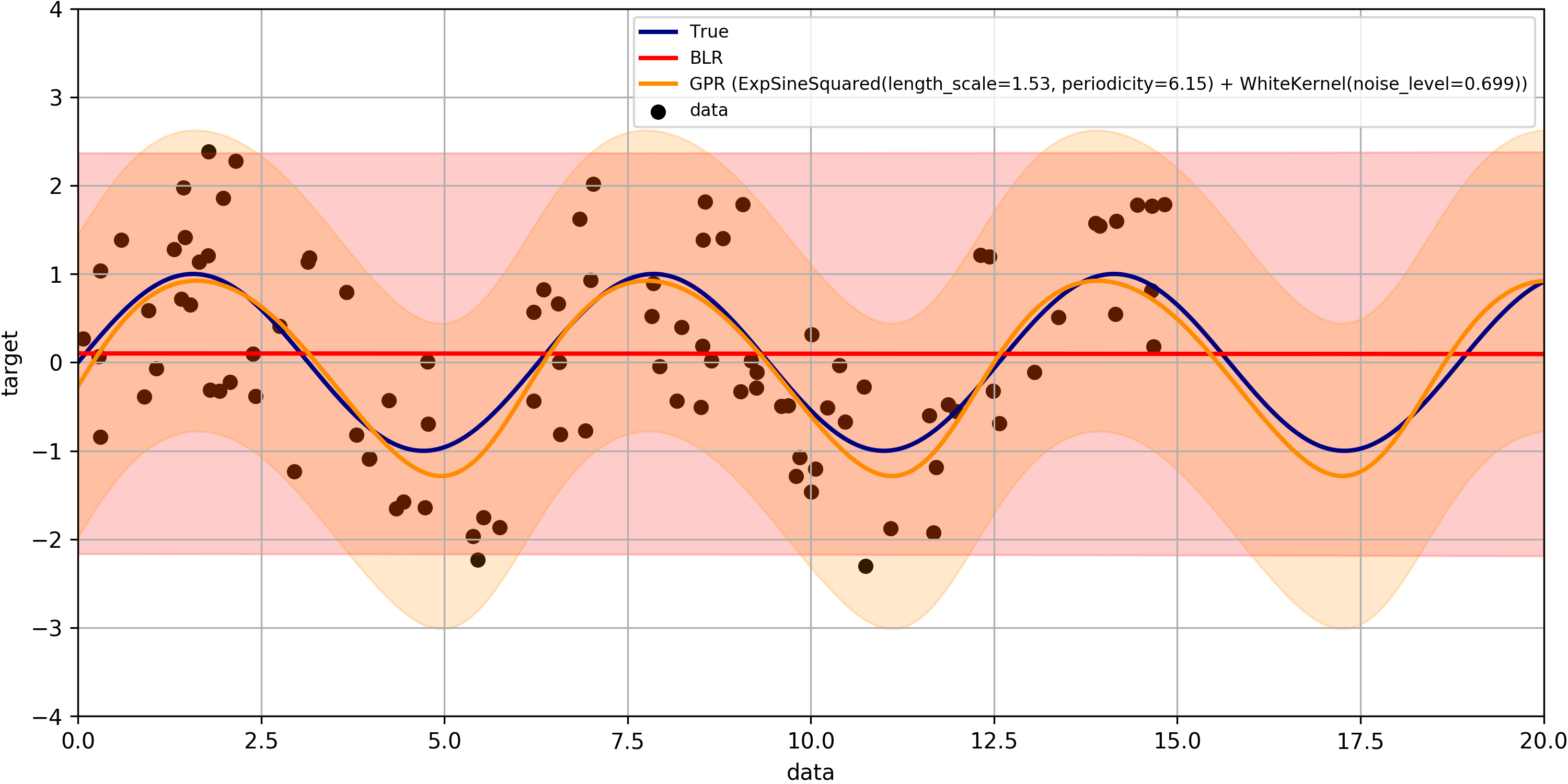
Usage for regression problems
The mlpaper package can also be applied to a regression problem with:
import mlpaper.regression as btr

full_tbl = btr.just_benchmark(X_train, y_train, X_test, y_test, regressors, STD_REGR_LOSS, "iid", pairwise_CI=True)
Here we have used pairwise_CI=True which makes the confidence intervals based on the uncertainty of the loss difference to the reference method rather than a confidence interval on the actual loss.
Output
By extending the sklearn regression demo we can make simple formatted tables:
             MAE       p          MSE        p   NLL (nats)        p
BLR  0.96933(30)  0.0979  1.39881(67)   0.0665  1.58842(57)   0.9828
GPR  0.75(13)     0.0009  0.75(28)     <0.0001  1.27(12)     <0.0001
iid  0.96908         N/A  1.3982           N/A  1.5884           N/A
or in LaTeX:
\begin{tabular}{|l|Sr|Sr|Sr|}
\toprule
{}  &        {MAE} &     {p} &        {MSE} &      {p} & {NLL (nats)} &      {p} \\
\midrule
BLR &  0.96933(30) &  0.0979 &  1.39881(67) &   0.0665 &  1.58842(57) &   0.9828 \\
GPR &  0.75(13)    &  0.0009 &  0.75(28)    &  <0.0001 &  1.27(12)    &  <0.0001 \\
iid &  0.96908     &     N/A &  1.3982      &      N/A &  1.5884      &      N/A \\
\bottomrule
\end{tabular}
Installation
Only Python>=3.5 is officially supported, but older versions of Python likely work as well.
The core package itself can be installed with:
pip install mlpaperTo also get the dependencies for the demos in the README install with
pip install mlpaper[demo]Contributing
The following instructions have been tested with Python 3.7.4 on Mac OS (10.14.6).
Install in editable mode
First, define the variables for the paths we will use:
GIT=/path/to/where/you/put/repos
ENVS=/path/to/where/you/put/virtualenvs
Then clone the repo in your git directory $GIT:
cd $GIT
git clone https://github.com/rdturnermtl/mlpaper.git
Inside your virtual environments folder $ENVS, make the environment:
cd $ENVS
virtualenv mlpaper --python=python3.7
source $ENVS/mlpaper/bin/activate
Now we can install the pip dependencies. Move back into your git directory and run
cd $GIT/mlpaper
pip install -r requirements/base.txt
pip install -e .  # Install the package itself
Contributor tools
First, we need to setup some needed tools:
cd $ENVS
virtualenv mlpaper_tools --python=python3.7
source $ENVS/mlpaper_tools/bin/activate
pip install -r $GIT/mlpaper/requirements/tools.txt
To install the pre-commit hooks for contributing run (in the mlpaper_tools environment):
cd $GIT/mlpaper
pre-commit install
To rebuild the requirements, we can run:
cd $GIT/mlpaper

# Check if there any discrepancies in the .in files
pipreqs mlpaper/ --diff requirements/base.in
pipreqs tests/ --diff requirements/test.in
pipreqs demos/ --diff requirements/demo.in
pipreqs docs/ --diff requirements/docs.in

# Regenerate the .txt files from .in files
pip-compile-multi --no-upgrade
Generating the documentation
First setup the environment for building with Sphinx:
cd $ENVS
virtualenv mlpaper_docs --python=python3.7
source $ENVS/mlpaper_docs/bin/activate
pip install -r $GIT/mlpaper/requirements/docs.txt
Then we can do the build:
cd $GIT/mlpaper/docs
make all
open _build/html/index.html
Documentation will be available in all formats in Makefile. Use make html to only generate the HTML documentation.
Running the tests
The tests for this package can be run with:
cd $GIT/mlpaper
./local_test.sh
The script creates an environment using the requirements found in requirements/test.txt. A code coverage report will also be produced in $GIT/mlpaper/htmlcov/index.html.
Deployment
The wheel (tar ball) for deployment as a pip installable package can be built using the script:
cd $GIT/mlpaper/
./build_wheel.sh
Links
The source is hosted on GitHub.
The documentation is hosted at Read the Docs.
Installable from PyPI.
License
This project is licensed under the Apache 2 License - see the LICENSE file for details.
Release history Release notifications | RSS feed


Download files
Download the file for your platform. If you're not sure which to choose, learn more about installing packages.
Source Distribution
File details
Details for the file mlpaper-0.0.3.tar.gz.
File metadata
- Download URL: mlpaper-0.0.3.tar.gz
- Upload date:
- Size: 53.3 kB
- Tags: Source
- Uploaded using Trusted Publishing? No
- Uploaded via: twine/3.1.1 pkginfo/1.5.0.1 requests/2.24.0 setuptools/47.3.1 requests-toolbelt/0.9.1 tqdm/4.46.1 CPython/3.7.4
File hashes
| Algorithm | Hash digest | |
|---|---|---|
| SHA256 |
525add6a45c5979fbfe26172838590e66eedf6e80d8d1438102f3649e210320a
|
|
| MD5 |
cab6b337209373d2f47b1492c74187e0
|
|
| BLAKE2b-256 |
0dcbec9bea40e20dfbd335b27f11e55bc291e7f6d6dd3c477cdf2e813b698122
|


