
MLVTK 

A loss surface visualization tool
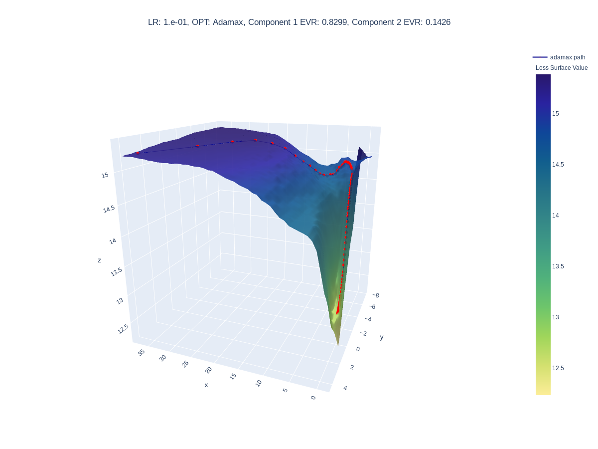
Simple DNN trained on MNIST data set, using Adamax optimizer

Simple DNN trained on MNIST, using SGD optimizer
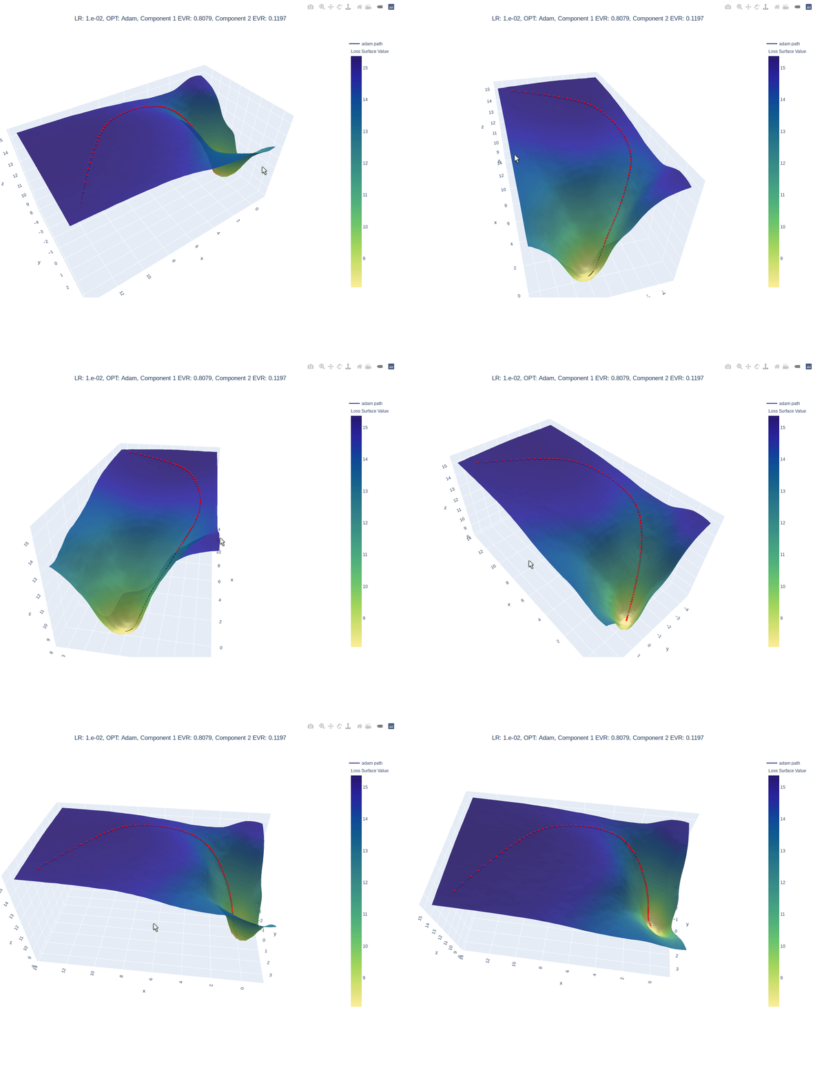
Simple DNN trained on MNIST, using Adam optimizer
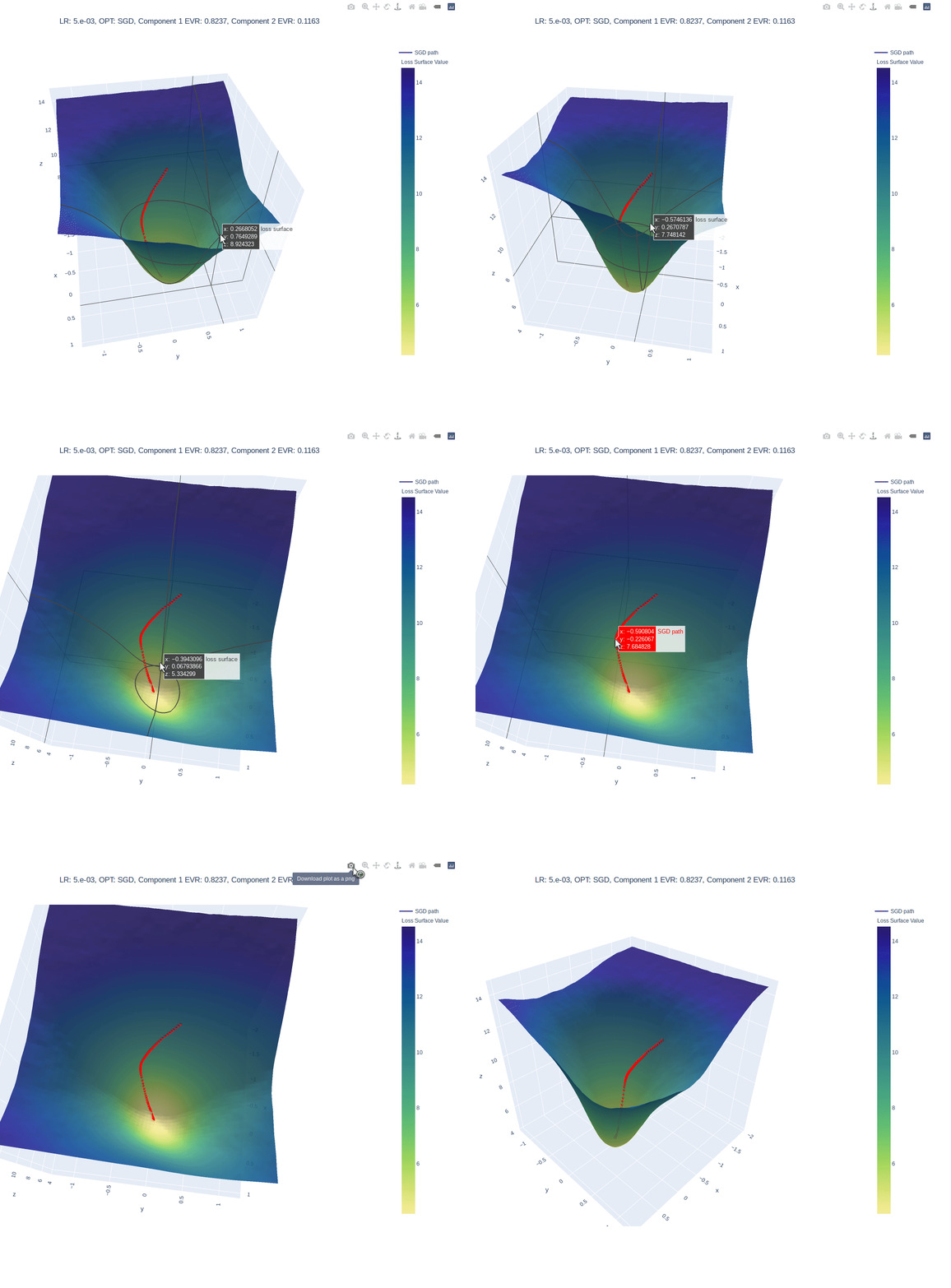
Simple DNN trained on MNIST, using SGD optimizer
Why?
- :shipit: Simple: A single line addition is all that is needed.
- :question: Informative: Gain insight into what your model is seeing.
- :notebook: Educational: See how your hyper parameters and architecture impact your models perception.
Quick Start
| Requires | version |
|---|---|
| python | >= 3.6.1 |
| tensorflow | >= 2.3.1, < 2.4.2 |
| plotly | >=4.9.0 |
Install locally (Also works in google Colab!):
pip install mlvtk
Optionally for use with jupyter notebook/lab:
Notebook
pip install "notebook>=5.3" "ipywidgets==7.5"
Lab
pip install jupyterlab "ipywidgets==7.5"

# Basic JupyterLab renderer support
jupyter labextension install jupyterlab-plotly@4.10.0

# OPTIONAL: Jupyter widgets extension for FigureWidget support
jupyter labextension install @jupyter-widgets/jupyterlab-manager plotlywidget@4.10.0
Basic Example
from mlvtk.base import Vmodel
import tensorflow as tf
import numpy as np

# NN with 1 hidden layer
inputs = tf.keras.layers.Input(shape=(None,100))
dense_1 = tf.keras.layers.Dense(50, activation='relu')(inputs)
outputs = tf.keras.layers.Dense(10, activation='softmax')(dense_1)
_model = tf.keras.Model(inputs, outputs)

# Wrap with Vmodel
model = Vmodel(_model)
model.compile(optimizer=tf.keras.optimizers.SGD(),
loss=tf.keras.losses.CategoricalCrossentropy(), metrics=['accuracy'])

# All tf.keras.(Model/Sequential/Functional) methods/properties are accessible
# from Vmodel

model.summary()
model.get_config()
model.get_weights()
model.layers

# Create random example data
x = np.random.rand(3, 10, 100)
y = np.random.randint(9, size=(3, 10, 10))
xval = np.random.rand(1, 10, 100)
yval = np.random.randint(9, size=(1,10,10))

# Only difference, model.fit requires validation_data (tf.data.Dataset, or
# other container
history = model.fit(x, y, validation_data=(xval, yval), epochs=10, verbose=0)

# Calling model.surface_plot() returns a plotly.graph_objs.Figure
# model.surface_plot() will attempt to display the figure inline

fig = model.surface_plot()

# fig can save an interactive plot to an html file,
fig.write_html("surface_plot.html")

# or display the plot in jupyter notebook/lab or other compatible tool.
fig.show()
1 maintainer

Release files for mlvtk 1.0.3
For a detailed explanation of source distributions (sdists) and built distributions (wheels), please see the package formats documentation.
Source distribution (sdist)
| File | Size | Uploaded | |
|---|---|---|---|
| mlvtk-1.0.3.tar.gz | 13.5 kB | Details |
Built distribution (wheel)
| File | Interpreter | ABI | Platform | Reset |
|---|---|---|---|---|
| mlvtk-1.0.3-py3-none-any.whl | Python 3 | none | any | Details |
Total release size: 27.6 kB
Release files / mlvtk-1.0.3.tar.gz
| Download URL | mlvtk-1.0.3.tar.gz |
|---|---|
| Size | 13.5 kB |
| Tags | Source |
|
SHA-256 checksum How to use checksums |
d4bc51c15ba23f6e442cfb22a7b7dda92b6629ab870a308012cbe46b346f7155
|
|
BLAKE2b-256 checksum How to use checksums |
76651ff5bf340f4041e424e10a4b4cf946e17fdf2657c46a6f13bc7c8352e93c
|
| Upload date | |
|
Uploaded using Trusted Publishing? What is trusted publishing? |
No |
| Uploaded via |
poetry/1.1.2 CPython/3.8.6 Linux/5.11.6-artix1-1
|
Release files / mlvtk-1.0.3-py3-none-any.whl
| Download URL | mlvtk-1.0.3-py3-none-any.whl |
|---|---|
| Size | 14.1 kB |
| Tags | Python 3 |
|
SHA-256 checksum How to use checksums |
d181c91666994172cd3fce149b8bcb1cce7a330b6ffb3778feeb69b548c91ba3
|
|
BLAKE2b-256 checksum How to use checksums |
a7df114ff83effd0e88ba6f113f46ba71ce5ed64adb900e878a4a7e16a226a80
|
| Upload date | |
|
Uploaded using Trusted Publishing? What is trusted publishing? |
No |
| Uploaded via |
poetry/1.1.2 CPython/3.8.6 Linux/5.11.6-artix1-1
|














