
mplstereonet
mplstereonet provides lower-hemisphere equal-area and equal-angle stereonets for matplotlib.
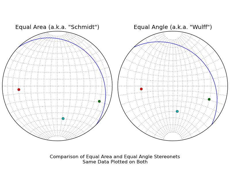
What’s New
Polar overlays and arbitrary rotated grid overlays. See https://mplstereonet.readthedocs.io/en/latest/examples/polar_overlay.html for more details.
Numerous bugfixes and compatibility with recent versions of matplotlib and numpy
Install
mplstereonet can be installed from PyPi using pip by:
pip install mplstereonet
Alternatively, you can download the source and install locally using (from the main directory of the repository):
python setup.py install
If you’re planning on developing mplstereonet or would like to experiment with making local changes, consider setting up a development installation so that your changes are reflected when you import the package:
python setup.py develop
Basic Usage
In most cases, you’ll want to import mplstereonet and then make an axes with projection="stereonet" (By default, this is an equal-area stereonet). Alternately, you can use mplstereonet.subplots, which functions identically to matplotlib.pyplot.subplots, but creates stereonet axes.
As an example:
import matplotlib.pyplot as plt
import mplstereonet

fig = plt.figure()
ax = fig.add_subplot(111, projection='stereonet')

strike, dip = 315, 30
ax.plane(strike, dip, 'g-', linewidth=2)
ax.pole(strike, dip, 'g^', markersize=18)
ax.rake(strike, dip, -25)
ax.grid()

plt.show()
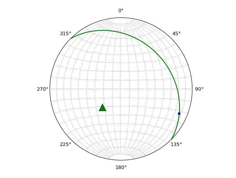
Planes, lines, poles, and rakes can be plotted using axes methods (e.g. ax.line(plunge, bearing) or ax.rake(strike, dip, rake_angle)).
All planar measurements are expected to follow the right-hand-rule to indicate dip direction. As an example, 315/30S would be 135/30 following the right-hand rule.
Density Contouring
mplstereonet also provides a few different methods of producing contoured orientation density diagrams.
The ax.density_contour and ax.density_contourf axes methods provide density contour lines and filled density contours, respectively. “Raw” density grids can be produced with the mplstereonet.density_grid function.
As a basic example:
import matplotlib.pyplot as plt
import numpy as np
import mplstereonet

fig, ax = mplstereonet.subplots()

strike, dip = 90, 80
num = 10
strikes = strike + 10 * np.random.randn(num)
dips = dip + 10 * np.random.randn(num)

cax = ax.density_contourf(strikes, dips, measurement='poles')

ax.pole(strikes, dips)
ax.grid(True)
fig.colorbar(cax)

plt.show()
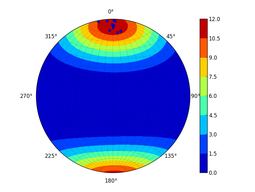
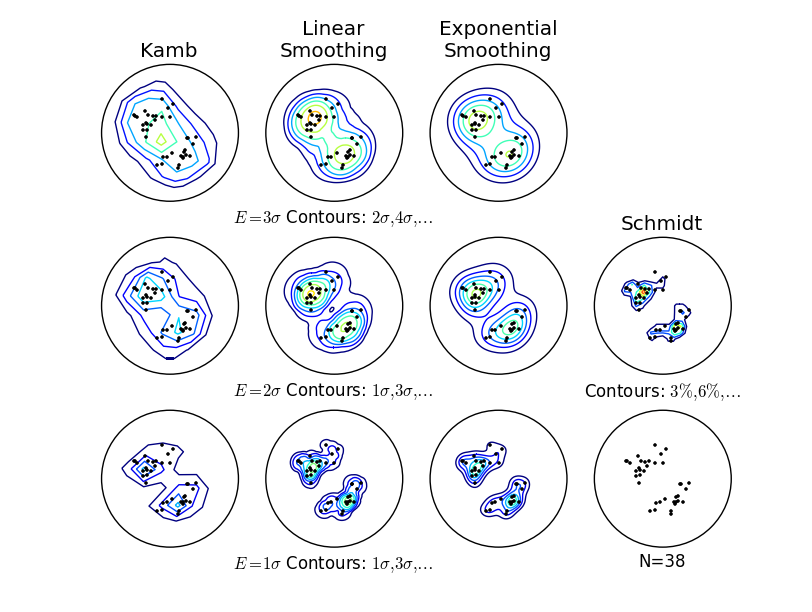
By default, a modified Kamb method with exponential smoothing [Vollmer1995] is used to estimate the orientation density distribution. Other methods (such as the “traditional” Kamb [Kamb1956] and “Schmidt” (a.k.a. 1%) methods) are available as well. The method and expected count (in standard deviations) can be controlled by the method and sigma keyword arguments, respectively.
Utilities
mplstereonet also includes a number of utilities to parse structural measurements in either quadrant or azimuth form such that they follow the right-hand-rule.
For an example, see parsing_example.py:
Parse quadrant azimuth measurements
"N30E" --> 30.0
"E30N" --> 60.0
"W10S" --> 260.0
"N 10 W" --> 350.0

Parse quadrant strike/dip measurements.
Note that the output follows the right-hand-rule.
"215/10" --> Strike: 215.0, Dip: 10.0
"215/10E" --> Strike: 35.0, Dip: 10.0
"215/10NW" --> Strike: 215.0, Dip: 10.0
"N30E/45NW" --> Strike: 210.0, Dip: 45.0
"E10N   20 N" --> Strike: 260.0, Dip: 20.0
"W30N/46.7 S" --> Strike: 120.0, Dip: 46.7

Similarly, you can parse rake measurements that don't follow the RHR.
"N30E/45NW 10NE" --> Strike: 210.0, Dip: 45.0, Rake: 170.0
"210 45 30N" --> Strike: 210.0, Dip: 45.0, Rake: 150.0
"N30E/45NW raking 10SW" --> Strike: 210.0, Dip: 45.0, Rake: 10.0
Additionally, you can find plane intersections and make other calculations by combining utility functions. See plane_intersection.py and parse_anglier_data.py for examples.
Analysis
mplstereonet contains orientation data analysis methods, as well as plotting functionality. For example, you can fit planes to girdles or fit a pole to points, identify different modes of conjugate sets of faults, or calculate flattening values for Flinn plots.
Full Documentation
Full documentation is available at https://mplstereonet.readthedocs.io/en/latest/mplstereonet.html
References
Kamb, 1959. Ice Petrofabric Observations from Blue Glacier, Washington, in Relation to Theory and Experiment. Journal of Geophysical Research, Vol. 64, No. 11, pp. 1891–1909.
Vollmer, 1995. C Program for Automatic Contouring of Spherical Orientation Data Using a Modified Kamb Method. Computers & Geosciences, Vol. 21, No. 1, pp. 31–49.
1 maintainer

Metadata
1 maintainer
Release files for mplstereonet 0.6.3
For a detailed explanation of source distributions (sdists) and built distributions (wheels), please see the package formats documentation.
Source distribution (sdist)
| File | Size | Uploaded | |
|---|---|---|---|
| mplstereonet-0.6.3.tar.gz | 1.7 MB | Details |
Release files / mplstereonet-0.6.3.tar.gz
| Download URL | mplstereonet-0.6.3.tar.gz |
|---|---|
| Size | 1.7 MB |
| Tags | Source |
|
SHA-256 checksum How to use checksums |
2ce630b14973a0b2f7d65cabb8d03fada2a8fda8b9b922d4cf335ecfcb442372
|
|
BLAKE2b-256 checksum How to use checksums |
ae4152c87d0c1b0799f5948f31bf63bc56350db9da9d1e8b6f56fa7ebe315069
|
| Upload date | |
|
Uploaded using Trusted Publishing? What is trusted publishing? |
No |
| Uploaded via |
twine/4.0.2 CPython/3.10.13
|














