Python library for large-scale targeted metabolomics.

Project description


ms-mint: The Python library for data scientists doing large-scale metabolomics
The ms-mint library includes a range of functions for processing LCMS data from targeted metabolomics experiments, and it is particularly well-suited for handling large amounts of data (10,000+ files). To use ms-mint, you provide it with a target list of the specific metabolites you want to analyze, as well as the names of the mass spectrometry files containing the data. ms-mint then extracts peak intensities and other relevant information from the data, allowing you to gain insights into the concentrations and profiles of the metabolites in your samples. This information can be used to identify biomarkers, which are indicators of disease or other physiological changes that can be used in the development of diagnostic tests or other medical applications. ms-mint can be used in Python scripts, interactively in Jupyter Notebooks, or with the web-app (info below).
News
Starting with version 1.0.0, we have updated the installation setup to use pyproject.toml. Additionally, each release of the repository will now be assigned a DOI to facilitate citation of the software.
Installation
pip install ms-mint
Documentation
The code documentation can be accessed here.
ms-mint application with graphical user iterface (GUI)
MINT has been split into the Python library and the app. This repository contains the Python library. For the app follow this link.
Publications that used ms-mint
-
Brown K, Thomson CA, Wacker S, Drikic M, Groves R, Fan V, et al. Microbiota alters the metabolome in an age- and sex- dependent manner in mice. Nat Commun. 2023;14: 1348.
-
Ponce LF, Bishop SL, Wacker S, Groves RA, Lewis IA. SCALiR: A Web Application for Automating Absolute Quantification of Mass Spectrometry-Based Metabolomics Data. Anal Chem. 2024;96: 6566–6574.
-
Groves RA, Chan CCY, Wildman SD, Gregson DB, Rydzak T, Lewis IA. Rapid LC-MS assay for targeted metabolite quantification by serial injection into isocratic gradients. Anal Bioanal Chem. 2023 Jan;415(2):269-276. doi: 10.1007/s00216-022-04384-x. Epub 2022 Nov 28. PMID: 36443449; PMCID: PMC9823034.
Contributions
All contributions, bug reports, code reviews, bug fixes, documentation improvements, enhancements, and ideas are welcome. Before you modify the code please reach out to us using the issues page.
Code standards
The project follows PEP8 standard and uses Black and Flake8 to ensure a consistent code format throughout the project.
Usage
To use the main class of the ms-mint library, you can import it into your code with the following command:
from ms_mint.Mint import Mint
This will import a lightweight version of the class with the essential functionality. If you want to use the ms-mint tool interactively in a Jupyter Notebook or JupyterLab, you can import the class with the following command:
from ms_mint.notebook import Mint
This version of the class is designed specifically for use in Jupyter notebooks and includes additional functions. Once you have imported the appropriate version of the class, you can create an instance of the Mint class and use its methods to process your data.
ms-mint in JupyterLab, or the Jupyter Notebook
In the JupyterLab you would first instantiate the main class and then load a number of mass-spectrometry (MS) files and a target list.
%pylab inline
from ms_mint.notebook import Mint
mint = Mint()
Data extraction
Load files
You can import files simply by assigning a list to the Mint.ms_files attribute.
mint.ms_files = [
    './input/EC_B2.mzXML',
    './input/EC_B1.mzXML',
    './input/CA_B1.mzXML',
    './input/CA_B4.mzXML',
    './input/CA_B2.mzXML',
    './input/CA_B3.mzXML',
    './input/EC_B4.mzXML',
    './input/EC_B3.mzXML',
    './input/SA_B4.mzML',
    './input/SA_B2.mzML',
    './input/SA_B1.mzML',
    './input/SA_B3.mzML'
]
Or you can use the Mint.load_files() method which supports a string with regular expressions. The files in the previous function you could load with:
mint.load_files('./input/*.*')
This has the advantage that you can wildcards and you can chain your commands. For examle like this:
mint.load_files('./input/*.*').load_targets('targets.csv').run()
Load target list
Then you load the target definitions from a file the load_targets method is used:
mint.load_targets('targets.csv')

mint.targets
>>>    peak_label    mz_mean  mz_width       rt  rt_min  rt_max  rt_unit  intensity_threshold target_filename
    0    Arabitol  151.06050        10  4.92500    4.65    5.20      min                    0     targets.csv
    1    Xanthine  151.02585        10  4.37265    4.18    4.53      min                    0     targets.csv
    2   Succinate  117.01905        10  2.04390    0.87    2.50      min                    0     targets.csv
    3   Urocanate  137.03540        10  4.41500    4.30    4.60      min                    0     targets.csv
    4  Mevalonate  147.06570        10  3.00000    1.70    4.30      min                    0     targets.csv
    5  Nicotinate  122.02455        10  3.05340    2.75    3.75      min                    0     targets.csv
    6  Citrulline  174.08810        10  8.40070    8.35    8.50      min                    0     targets.csv
The retention time can be specified in minutes (rt_unit = 'min') or seconds (rt_unit = 's'). Mint will convert the values to SI unit seconds.
You can also prepare a pandas.DataFrame with the column names as shown above and assign it directly to the Mint.targets attribute:
mint.targets = my_targets_dataframe
Run data extraction
When filenames and targets are loaded, the processing can be started by calling the run() method:
mint.run() # Use mint.run(output_fn='results') for many files to prevent memory issues.
Then the results will be stored in the results attribute:
mint.results
>>>
...
Processing a large number of files
If you want to process a large number of files, you should provide an output filename. Then the results are written directly to that file instead of being stored in memory.
mint.run(fn='my-mint-output.csv')
Optimize retention times
If you only have retention time (Rt) values for your targets, or if the Rt values you have are not accurate, you can use the mint.opt.rt_min_max() function from the ms-mint library to generate better values for the rt_min and rt_max parameters. These parameters define the range of retention times within which ms-mint will search for peaks corresponding to your targets. By optimizing these values, you can improve the accuracy and reliability of your results.
To use the mint.opt.rt_min_max() function, you will need to provide it with a list of retention times for your targets and the names of the mass spectrometry files containing your data. The function will then search through the data to find the optimal rt_min and rt_max values, which you can use to refine your analysis. You can then use these optimized values in conjunction with the other functions and methods of the Mint class to process and analyze your data.
Now, we can run the peak optimization with:
mint.opt.rt_min_max(
    fns=[...]
    peak_labels=['Xanthine', 'Succinate', 'Citrulline'],
    plot=True, rel_height=0.7, sigma=50, col_wrap=1, aspect=3,
    height=4
)
The mint.opt.rt_min_max() function in the ms-mint library allows you to optimize the rt_min and rt_max values for your analysis. These values define the range of retention times within which ms-mint will search for peaks corresponding to your targets. By optimizing these values, you can improve the accuracy and reliability of your results.
If you do not provide a list of peak_labels to the mint.opt.rt_min_max() function, it will run the optimization for all metabolites. Similarly, if you do not provide a list of filenames for the fn parameter, the function will use all of the files currently loaded into mint.ms_files. It is generally recommended to use a maximum of 20-40 files for the optimization process. If you have run a set of standards along with your samples (which is highly recommended), you can use the standard files to perform the optimization.
After running the optimization, it is a good idea to perform a manual fine-tuning of the rt_min and rt_max values, especially for complicated peaks (peaks with multiple components, noisy peaks, etc.). You can use the mint.plot.peak_shapes() function to visualize the peak shapes and identify any areas that may require further attention.

The black lines indicates the average intensity across all files used for the optimization. The orange dotted lines show the shape of the gaussian function used to weight the mean intensities for peak selection. The orange horizontal lines indicate the peak width and the blue xs show the identified peak maxima. The green shaded areas show the Rt ranges which were selected by the algorithm.
Then we apply the changes and plot the new peak shapes:
mint.run()
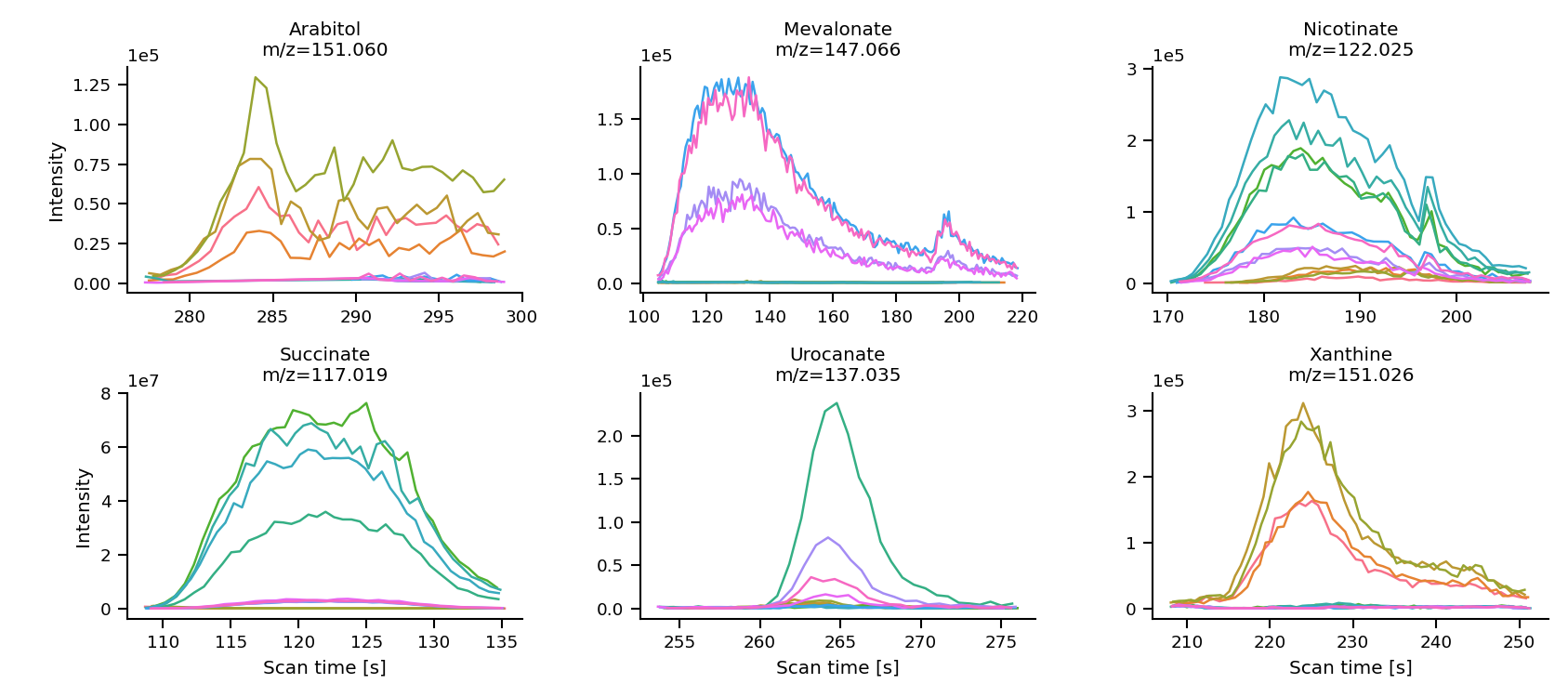
mint.plot.peak_shapes(col_wrap=3)

As you can see, the shapes of Xanthine, Succinate, Citrulline look much better.
Plotting and data exploration
The Mint class has a few convenient methods to visualize and explore the processed data. The results can be viewed directly in JupyterLab or stored to files using matplotlib and seaborn syntax. The figures are matplotlib objects and can be easily customised.
Plot peak shapes
mint.plot.peak_shapes(col_wrap = 3)
The method uses seaborn sns.relplot() function and keyword arguments are passed on.
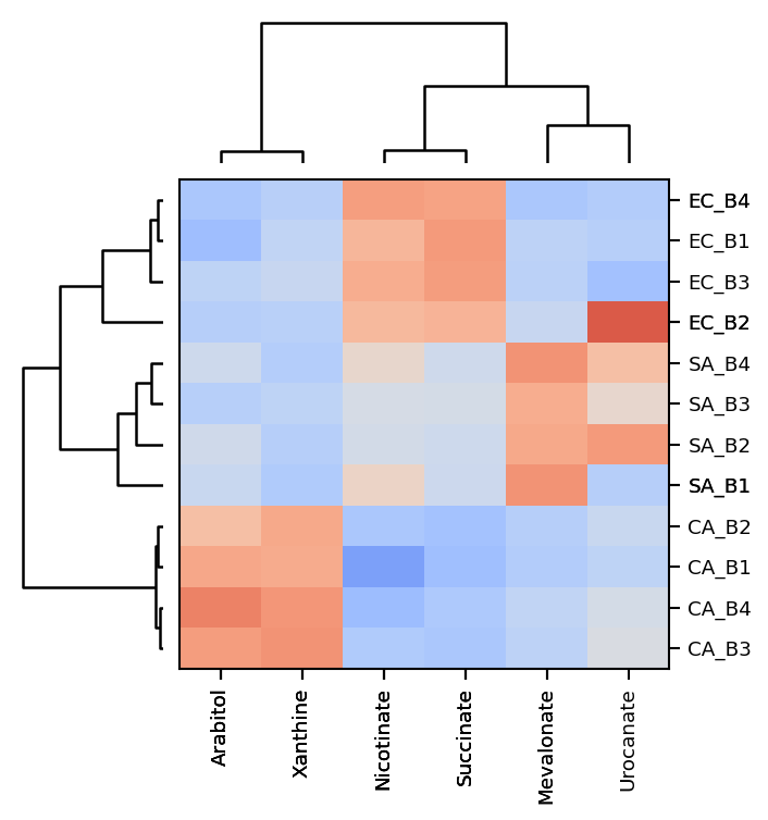
Hierarchical clustering
Mint ca be used to cluster the extracted data. An agglomerative hierarchical clustering is a bottom-up clustering technique where each data point starts as its own cluster and then are merged with other clusters in a hierarchical manner based on their proximity or similarity until a single cluster is formed or a specified stopping criteria is met. The proximity is usually determined by a distance metric, such as Euclidean distance, and the similarity is usually determined by a linkage function, such as ward linkage or complete linkage. The result is a tree-like representation called a dendrogram, which can be used to determine the number of clusters and the cluster assignments of the data points.
Mint uses scipy.spartial.distance to generate the distance matrix and scipy.cluster.hierarchy.linkage to perform the clustering. By default a 'cosine' metric is used to calculate the distances. Distances between row vectors and column vectors respectively can also be done using different metrics for each set. To do so a tuple with the names of the metrics has to be provided: mint.hierarchical_clustering(metric=("euclidean", "cosine").
Before clustering the data can be transformed and scaled. By default log2p1(x) = log_2(x+1) is used to transform the data and the standard scaler (z-scores) is used to normalize the variables for each target.
mint.plot.hierarchical_clustering(
    data=None,  # Optional, dataframe. if None, mint.crosstab(targets_var) is executed to generate the data.
    peak_labels=None,  # List of targets to include
    ms_files=None,  # List of filenames to include
    title=None,  # Title to add to the figure
    figsize=(8, 8),  # Figure size
    targets_var="peak_max",  # Data variable to plot if data is None.
    vmin=-3,  # Minimum value for color bar
    vmax=3,  # Maximum value for color bar
    xmaxticks=None,  # Maximum number of x-ticks to display
    ymaxticks=None,  # Maximum number of y-ticks to display
    transform_func="log2p1",  # Transformation to use before scaling and clustering
    scaler_ms_file=None,  # Experimental
    scaler_peak_label="standard",  # Scaler to use to normalize the data before clustering
    metric="cosine",  # Metric either a string or a 2-tuple of strings
    transform_filenames_func="basename",  # Transformation function to shorten filenames
    transposed=False,  # Transpose the plot
    top_height=2,  # Height of the top-dendrogram
    left_width=2,  # Width of the left-dendrogram
    cmap=None  # Name of a matplotlib color map
)
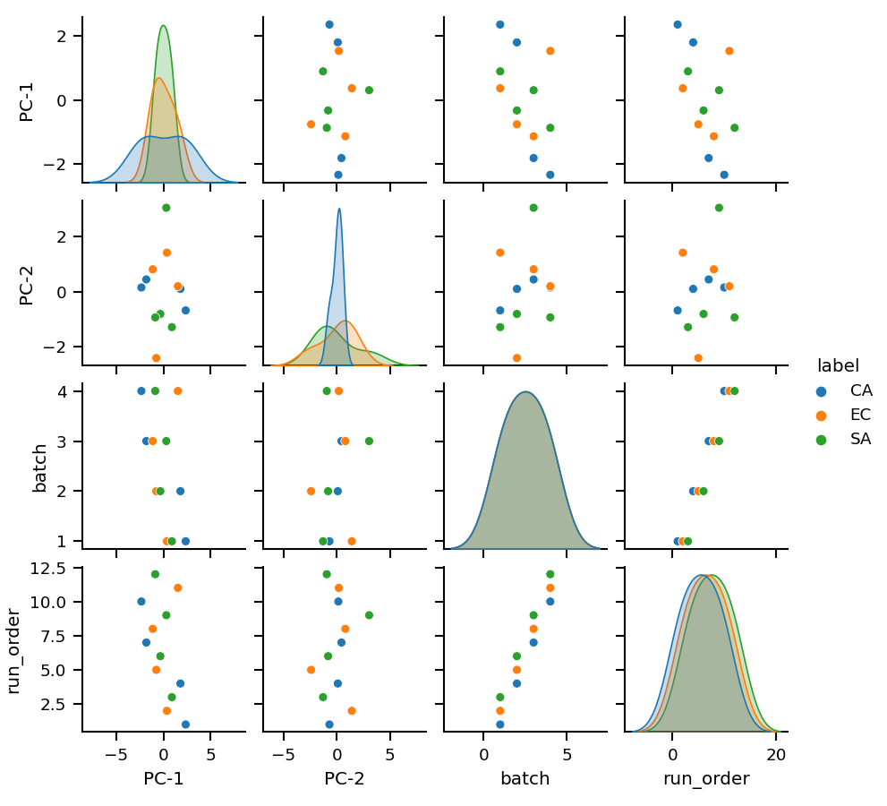
Principal Components Analysis
Principal Component Analysis (PCA) is a widely used statistical technique for dimensionality reduction. It transforms the original high-dimensional data into a new set of linearly uncorrelated variables, called Principal Components (PCs), that capture the maximum variance in the data. The first PC accounts for the largest variance in the data, the second PC for the second largest variance, and so on. PCA is commonly used for data visualization, data compression, and noise reduction. By reducing the number of dimensions in the data, PCA allows us to more easily identify patterns and relationships in the data.
Before clustering the data can be transformed and scaled. By default log2p1(x) = log_2(x+1) is used to transform the data and the standard scaler (z-scores) is used to normalize the variables for each target.
mint.pca.run(n_components=5)
After running the PCA the results can be plotted with:
mint.pca.plot.pairplot(n_components=5, interactive=False)
FAQ
What is a target list
A target list is a pandas dataframe with specific columns.
- peak_label: string, Label of the peak (must be unique).
- mz_mean: numeric value, theoretical m/z value of the target ion to extract.
- mz_width: numeric value, width of the peak in [ppm]. It is used to calculate the width of the mass window according to the formula:
Δm = m/z * 1e-6 * mz_width. - rt: numeric value, (optional), expected time of the peak. This value is not used during processing, but it can inform the peak optimization procedure.
- rt_min: numeric value, starting time for peak integration.
- rt_max: numeric value, ending time for peak integration.
- rt_unit: one of
sorminfor seconds or minutes respectively. - intensity_threshold: numeric value (>=0), minimum intensity value to include, serves as a noise filter. We recommend setting this to 0.
- target_filename: string (optional), name of the target list file. It is not used for processing, just to keep track of what files were used.
The target list can be stored as csv or Excel file.
What input files can be used
ms_mint can be used with mzXML, mzML, mzMLb and experimental formats in .feather and .parquet format.
Which properties does ms-mint extract
Parameters from target list
- ms_file: Filename of MS-file
- peak_label: From target list
- mz_mean: From target list
- mz_width: From target list
- rt: From target list
- rt_min: From target list
- rt_max: From target list
- rt_unit: Unit of retention times, default is s (seconds), from [s, min]
- intensity_threshold: From target list
- target_filename: From target list
Results columns
- peak_area: The sum of all intensities in the extraction window
- peak_area_top3: The average of the 3 largest intensities in the extraction window
- peak_n_datapoints: Number of datapoints
- peak_max: Intensity of peak maximum
- peak_rt_of_max: Retentiontime of peak maximum
- peak_min: Minimum peak intensity (offset)
- peak_median: Median of all intensities
- peak_mean: Average of all intensities
- peak_delta_int: Difference between first and last intensity
- peak_shape_rt: Array of retention times
- peak_shape_int: Array of projected intensities
- peak_mass_diff_25pc: 25th percentile between mz_mean minus m/z values of all datapoints
- peak_mass_diff_50pc: Median between mz_mean minus m/z values of all datapoints
- peak_mass_diff_75pc: 75th percentile between mz_mean minus m/z values of all datapoints
- peak_score: Score of peak quality (experimental)
- total_intensity: Sum of all intensities in the file
- ms_path: Path of the MS-file
- ms_file_size: Size of the MS-file in MB
Release history Release notifications | RSS feed


Download files
Download the file for your platform. If you're not sure which to choose, learn more about installing packages.
Source Distribution
Built Distribution
Filter files by name, interpreter, ABI, and platform.
If you're not sure about the file name format, learn more about wheel file names.
Copy a direct link to the current filters
File details
Details for the file ms_mint-1.1.1.tar.gz.
File metadata
- Download URL: ms_mint-1.1.1.tar.gz
- Upload date:
- Size: 84.5 MB
- Tags: Source
- Uploaded using Trusted Publishing? No
- Uploaded via: twine/6.1.0 CPython/3.13.3
File hashes
| Algorithm | Hash digest | |
|---|---|---|
| SHA256 |
36231e81d01152a6d8bff36fc1aa883afbee3e668e554f4934f8af281d7877cb
|
|
| MD5 |
5e1e4ce2bfac055a9c6ec47b55a3022f
|
|
| BLAKE2b-256 |
d0d79e40c3b3e94b19c042035ee35e3050f90ac6ba6adaaf1b6f7c62802eac38
|
File details
Details for the file ms_mint-1.1.1-py3-none-any.whl.
File metadata
- Download URL: ms_mint-1.1.1-py3-none-any.whl
- Upload date:
- Size: 54.9 kB
- Tags: Python 3
- Uploaded using Trusted Publishing? No
- Uploaded via: twine/6.1.0 CPython/3.13.3
File hashes
| Algorithm | Hash digest | |
|---|---|---|
| SHA256 |
dc5410e8d82b30769220d3537666f8f6b3b114ea9f591b734d875a2c042cf1f5
|
|
| MD5 |
4a9d34f27634dde6d08bfb9757ff8311
|
|
| BLAKE2b-256 |
368056fece98112c009a3d6171046facd09d7d35f5d61e86e862a21b0c436e90
|


