A converter that takes a network (cnet, igraph, networkx, pathpy, ...) and creates a tikz-network for smooth integration into LaTeX.

Project description
network2tikz
| Module: | network2tikz |
|---|---|
| Date: | 07 November 2018 |
| Authors: | Jürgen Hackl |
| Contact: | hackl.j@gmx.at |
| License: | GNU GPLv3 |
| Version: | 0.1.8 |
This is network2tikz, a Python tool for converting network
visualizations into TikZ
(tikz-network)
figures, for native inclusion into your LaTeX documents.
network2tikz works with Python 3 and supports (currently) the
following Python network modules:
- cnet
- python-igraph
- networkx
- pathpy
- default node/edge lists
The output of network2tikz is
in tikz-network, a LaTeX
library that sits on top of TikZ,
which allows to visualize and modify the network plot for your
specific needs and publications.
Because you are not only getting an image of your network, but also the LaTeX source file, you can easily post-process the figures (e.g. adding drawings, texts, equations,...).
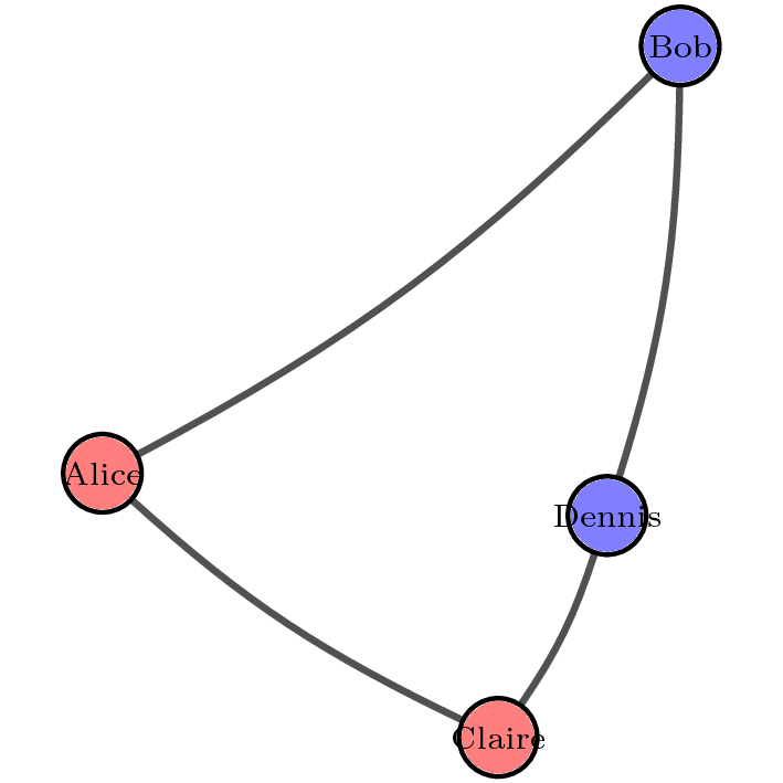
Since a picture is worth a thousand words a small example:
nodes = ['a','b','c','d']
edges = [('a','b'), ('a','c'), ('c','d'),('d','b')]
gender = ['f', 'm', 'f', 'm']
colors = {'m': 'blue', 'f': 'red'}

style = {}
style['node_label'] = ['Alice', 'Bob', 'Claire', 'Dennis']
style['node_color'] = [colors[g] for g in gender]
style['node_opacity'] = .5
style['edge_curved'] = .1

from network2tikz import plot
plot((nodes,edges),'network.tex',**style)
(see above) gives
\documentclass{standalone}
\usepackage{tikz-network}
\begin{document}
\begin{tikzpicture}
\clip (0,0) rectangle (6,6);
\Vertex[x=0.785,y=2.375,color=red,opacity=0.5,label=Alice]{a}
\Vertex[x=5.215,y=5.650,color=blue,opacity=0.5,label=Bob]{b}
\Vertex[x=3.819,y=0.350,color=red,opacity=0.5,label=Claire]{c}
\Vertex[x=4.654,y=2.051,color=blue,opacity=0.5,label=Dennis]{d}
\Edge[,bend=-8.531](a)(c)
\Edge[,bend=-8.531](c)(d)
\Edge[,bend=-8.531](d)(b)
\Edge[,bend=-8.531](a)(b)
\end{tikzpicture}
\end{document}
and looks like
Tweaking the plot is straightforward and can be done as part of your LaTeX workflow. The tikz-network manual contains multiple examples of how to make your plot look even better.
Installation
network2tikz is available from the Python Package Index, so simply type
pip install -U network2tikz
to install/update.
Usage
-
Generate, manipulation, and study of the structure, dynamics, and functions of your complex networks as usual, with your preferred python module.
-
Instead of the default plot functions (e.g.
igraph.plot()ornetworkx.draw()) invokenetwork2tikzbyplot(G,'mytikz.tex')
to store your network visualisation as the TikZ file
mytikz.tex. Load the module with:from network2tikz import plot
Advanced usage: Of course, you always can improve your plot by manipulating the generated LaTeX file, but why not do it directly in Python? To do so, all visualization options available in tikz-network are also implemented in
network2tikz. The appearance of the plot can be modified by keyword arguments (for a detailed explanation, please see below).my_style = {} plot(G,'mytikz.tex',**my_style)
The arguments follow the options available in the tikz-network library and are also explained in the tikz-network manual.
Additionally, if you are more interested in the final output and not only the
.texfile, usedplot(G,'mypdf.pdf')
to save your plot as a pdf, or
plot(G)
to create a temporal plot and directly show the result, i.e. similar to the matplotlib function
show(). Finally, you can also create a node and edge list, which can be read and easily modified (in a post-processing step) with tikz-network:plot(G,'mycsv.csv')
-
Note:
In order to compile the plot, make sure you have installed tikz-network!
-
Compile the figure or add the contents of
mytikz.texinto your LaTeX source code. With the optionstandalone=falseonly the TikZ figure will be saved, which can then be easily included in your LaTeX document via\input{/path/to/mytikz.tex}.
Simple example
For illustration purpose, a similar network as in the python-igraph tutorial is used. If you are using another Python network module, and like to follow this example, please have a look at the provided examples.
Create network object and add some edges.
import igraph
from network2tikz import plot

net = igraph.Graph([(0,1), (0,2), (2,3), (3,4), (4,2), (2,5), (5,0), (6,3),
                    (5,6), (6,6)],directed=True)
Adding node and edge properties.
net.vs["name"] = ["Alice", "Bob", "Claire", "Dennis", "Esther", "Frank", "George"]
net.vs["age"] = [25, 31, 18, 47, 22, 23, 50]
net.vs["gender"] = ["f", "m", "f", "m", "f", "m", "m"]
net.es["is_formal"] = [False, False, True, True, True, False, True, False,
                       False, False]
Already now the network can be plotted.
plot(net)
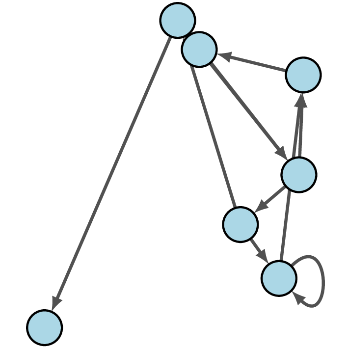
Per default, the node positions are assigned uniform random. In order to create a layout, the layout methods of the network packages can be used. Or the position of the nodes can be directly assigned, in form of a dictionary, where the key is the node id and the value is a tuple of the node position in x and y.
layout = {0: (4.3191, -3.5352), 1: (0.5292, -0.5292),
          2: (8.6559, -3.8008), 3: (12.4117, -7.5239),
          4: (12.7, -1.7069), 5: (6.0022, -9.0323),
          6: (9.7608, -12.7)}
plot(net,layout=layout)
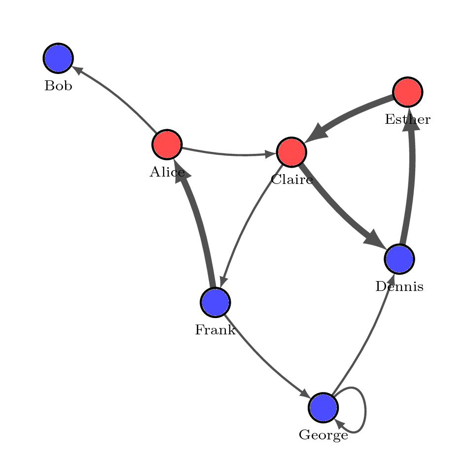
This should open an external pdf viewer showing a visual representation of the network, something like the one on the following figure:
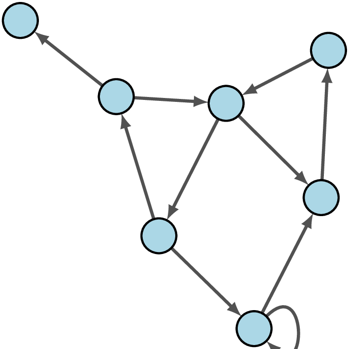
We can simply re-using the previous layout object here, but we also specified that we need a bigger plot (8 x 8 cm) and a larger margin around the graph to fit the self loop and potential labels (1 cm).
Note:
Per default, all size values are based on
cm, and all line widths are defined inptunits. With the general optionunitsthis can be changed, see below.
plot(net, layout=layout, canvas=(8,8), margin=1)
Note:
Instead of the command
marginsthe commandmargincan be used. Also instead ofcanvas,figure_sizeorbboxcan be used. For more information see table below.
In to keep the properties of the visual representation of your network
separate from the network itself. You can simply set up a Python
dictionary containing the keyword arguments you would pass to plot
and then use the double asterisk (**) operator to pass your specific
styling attributes to plot:
color_dict = {'m': 'blue', 'f': 'red'}
visual_style = {}
Node options
visual_style['vertex_size'] = .5
visual_style['vertex_color'] = [color_dict[g] for g in net.vs['gender']]
visual_style['vertex_opacity'] = .7
visual_style['vertex_label'] = net.vs['name']
visual_style['vertex_label_position'] = 'below'
Edge options
visual_style['edge_width'] = [1 + 2 * int(f) for f in net.es('is_formal')]
visual_style['edge_curved'] = 0.1
General options and plot command.
visual_style['layout'] = layout
visual_style['canvas'] = (8,8)
visual_style['margin'] = 1

plot(net,**visual_style)
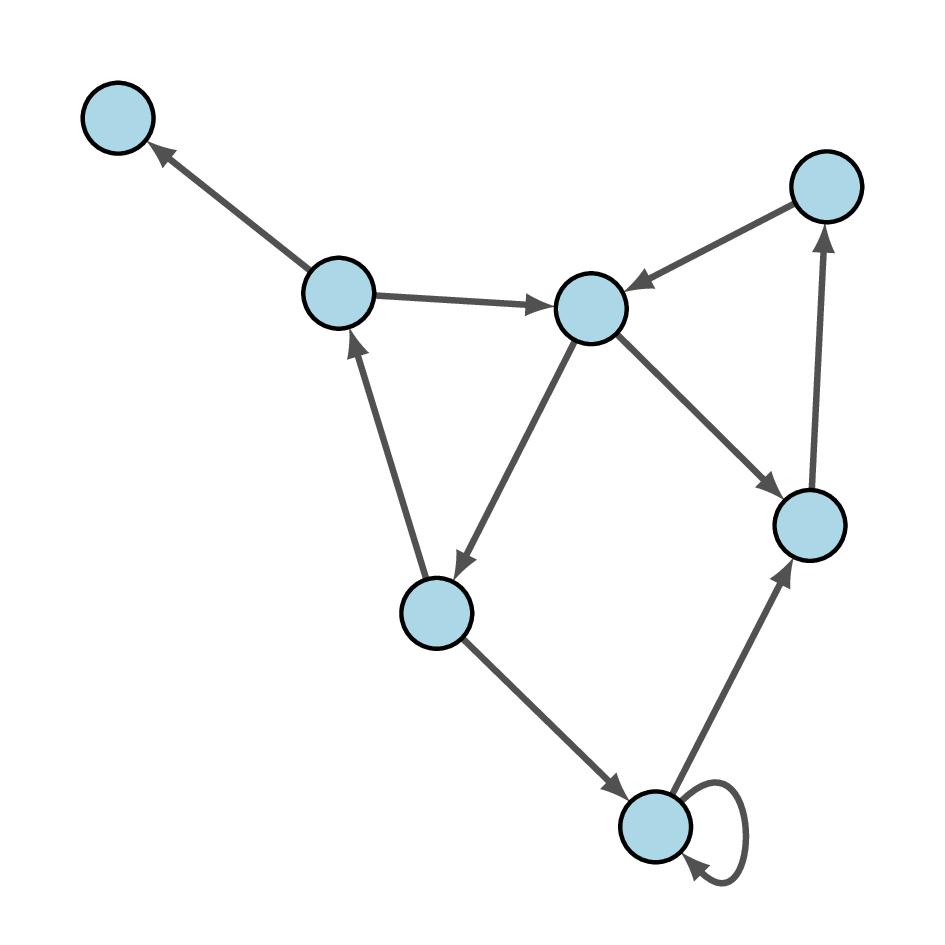
Beside showing the network, we can also generate the latex source
file, which can be used and modified later on. This is done by adding
the output file name with the ending '.tex'
plot(net,'network.tex',**visual_style)
\documentclass{standalone}
\usepackage{tikz-network}
\begin{document}
\begin{tikzpicture}
\clip (0,0) rectangle (8.0,8.0);
\Vertex[x=2.868,y=5.518,size=0.5,color=red,opacity=0.7,label=Alice,position=below]{a}
\Vertex[x=1.000,y=7.000,size=0.5,color=blue,opacity=0.7,label=Bob,position=below]{b}
\Vertex[x=5.006,y=5.387,size=0.5,color=red,opacity=0.7,label=Claire,position=below]{c}
\Vertex[x=6.858,y=3.552,size=0.5,color=blue,opacity=0.7,label=Dennis,position=below]{d}
\Vertex[x=7.000,y=6.419,size=0.5,color=red,opacity=0.7,label=Esther,position=below]{e}
\Vertex[x=3.698,y=2.808,size=0.5,color=blue,opacity=0.7,label=Frank,position=below]{f}
\Vertex[x=5.551,y=1.000,size=0.5,color=blue,opacity=0.7,label=George,position=below]{g}
\Edge[,lw=1.0,bend=-8.531,Direct](a)(b)
\Edge[,lw=1.0,bend=-8.531,Direct](a)(c)
\Edge[,lw=3.0,bend=-8.531,Direct](c)(d)
\Edge[,lw=3.0,bend=-8.531,Direct](d)(e)
\Edge[,lw=3.0,bend=-8.531,Direct](e)(c)
\Edge[,lw=1.0,bend=-8.531,Direct](c)(f)
\Edge[,lw=3.0,bend=-8.531,Direct](f)(a)
\Edge[,lw=1.0,bend=-8.531,Direct](f)(g)
\Edge[,lw=1.0,bend=-8.531,Direct](g)(g)
\Edge[,lw=1.0,bend=-8.531,Direct](g)(d)
\end{tikzpicture}
\end{document}
Instead of the tex file, a node and edge list can be generates, which can also be used with the tikz-network library.
plot(net,'network.csv',**visual_style)
The node list network_nodes.csv.
id,x,y,size,color,opacity,label,position
a,2.868,5.518,0.5,red,0.7,Alice,below
b,1.000,7.000,0.5,blue,0.7,Bob,below
c,5.006,5.387,0.5,red,0.7,Claire,below
d,6.858,3.552,0.5,blue,0.7,Dennis,below
e,7.000,6.419,0.5,red,0.7,Esther,below
f,3.698,2.808,0.5,blue,0.7,Frank,below
g,5.551,1.000,0.5,blue,0.7,George,below
The edge list network_edges.csv.
u,v,lw,bend,Direct
a,b,1.0,-8.531,true
a,c,1.0,-8.531,true
c,d,3.0,-8.531,true
d,e,3.0,-8.531,true
e,c,3.0,-8.531,true
c,f,1.0,-8.531,true
f,a,3.0,-8.531,true
f,g,1.0,-8.531,true
g,g,1.0,-8.531,true
g,d,1.0,-8.531,true
The plot function in detail
network2tikz.plot(network, filename=None, type=None, **kwds)
Parameters
-
network : network object
Network to be drawn. The network can be a 'cnet', 'networkx', 'igraph', 'pathpy' object, or a tuple of a node list and edge list.
-
filename : file, string or None, optional (default = None)
File or filename to save. The file ending specifies the output. i.e. is the file ending with '.tex' a tex file will be created; if the file ends with '.pdf' a pdf is created; if the file ends with '.csv', two csv files are generated (filename_nodes.csv and filename_edges.csv). If the filename is a tuple of strings, the first entry will be used to name the node list and the second entry for the edge list; and if no ending and no type is defined a temporary pdf file is compiled and shown.
-
type : str or None, optional (default = None)
Type of the output file. If no ending is defined trough the filename, the type of the output file can be specified by the type option. Currently the following output types are supported: 'tex', 'pdf', 'csv' and 'dat'.
-
kwds : keyword arguments, optional (default= no attributes)
Attributes used to modify the appearance of the plot. For details see below.
Keyword arguments for node styles
-
node_size: size of the node. The default is 0.6 cm. -
node_color: color of the nodes. The default is light blue. Colors can be specified either by common color names, or by 3-tuples of floats (ranging between 0 and 255 for the R, G and B components). -
node_opacity: opacity of the nodes. The default is 1. The range of the number lies between 0 and 1. Where 0 represents a fully transparent fill and 1 a solid fill. -
node_label: labels drawn next to the nodes. -
node_label_position: Per default the position of the label is in the center of the node. Classical Tikz commands can be used to change the position of the label. Instead, using such command, the position can be determined via an angle, by entering a number between -360 and 360. The origin (0) is the y axis. A positive number change the position counter clockwise, while a negative number make changes clockwise. -
node_label_distance: distance between the node and the label. -
node_label_color: color of the label. -
node_label_size: font size of the label. -
node_shape: shape of the vertices. Possibilities are: 'circle', 'rectangle', 'triangle', and any other Tikz shape -
node_style: Any other Tikz style option or command can be entered via the option style. Most of these commands can be found in the "TikZ and PGF Manual". Contain the commands additional options (e.g. shading = ball), then the argument for the style has to be between { } brackets. -
node_layer: the node can be assigned to a specific layer. -
node_label_off: is Boolean option which suppress all labels. -
node_label_as_id: is a Boolean option which assigns the node id as label. -
node_math_mode: is a Boolean option which transforms the labels into mathematical expressions without using the $ $ environment. -
node_pseudo: is a Boolean option which creates a pseudo node, where only the node name and the node coordinate will be provided.
Keyword arguments for edge styles
-
edge_width: width of the edges. The default unit is point (pt). -
edge_color: color of the edges. The default is gray. Colors can be specified either by common color names, or by 3-tuples of floats (ranging between 0 and 255 for the R, G and B components). -
edge_opacity: opacity of the edges. The default is 1. The range of the number lies between 0 and 1. Where 0 represents a fully transparent fill and 1 a solid fill. -
edge_curved: whether the edges should be curved. Positive numbers correspond to edges curved in a counter-clockwise direction, negative numbers correspond to edges curved in a clockwise direction. Zero represents straight edges. -
edge_label: labels drawn next to the edges. -
edge_label_position: Per default the label is positioned in between both nodes in the center of the line. Classical Tikz commands can be used to change the position of the label. -
edge_label_distance: The label position between the nodes can be modified with the distance option. Per default the label is centered between both nodes. The position is expressed as the percentage of the length between the nodes, e.g. of distance = 0.7, the label is placed at 70% of the edge length away of Vertex i. -
edge_label_color: color of the label. -
edge_label_size: font size of the label. -
edge_style: Any other Tikz style option or command can be entered via the option style. Most of these commands can be found in the "TikZ and PGF Manual". Contain the commands additional options (e.g. shading = ball), then the argument for the style has to be between { } brackets. -
edge_arrow_size: arrow size of the edges. -
edge_arrow_width: width of the arrowhead on the edge. -
edge_loop_size: modifies the length of the edge. The measure value has to be insert together with its units. Per default the loop size is 1 cm. -
edge_loop_position: The position of the self-loop is defined via the rotation angle around the node. The origin (0) is the y axis. A positive number change the loop position counter clockwise, while a negative number make changes clockwise. -
edge_loop_shape: The shape of the self-loop is defined by the enclosing angle. The shape can be changed by decreasing or increasing the argument value of the loop shape option. -
edge_directed: is a Boolean option which transform edges to directed arrows. If the network is already defined as directed network this option is not needed, except to turn off the direction for one or more edges. -
edge_math_mode: is a Boolean option which transforms the labels into mathematical expressions without using the $ $ environment. -
edge_not_in_bg: Per default, the edge is drawn on the background layer of the tikz picture. I.e. objects which are created after the edges appear also on top of them. To turn this off, the option edge_not_in_bg has to be enabled.
Keyword arguments for layout styles
NOTE: All layout arguments can be entered with or without 'layout_' at the
beginning, e.g. 'layout_iterations' is equal to 'iterations'
-
layout: dict or string , optional (default = None) A dictionary with the node positions on a 2-dimensional plane. The key value of the dict represents the node id while the value represents a tuple of coordinates (e.g. n = (x,y)). The initial layout can be placed anywhere on the 2-dimensional plane.Instead of a dictionary, the algorithm used for the layout can be defined via a string value. Currently, supported are:
-
Random layout, where the nodes are uniformly at random placed in the unit square. This algorithm can be enabled with the keywords: 'Random', 'random', 'rand', or None
-
Fruchterman-Reingold force-directed algorithm. In this algorithm, the nodes are represented by steel rings and the edges are springs between them. The attractive force is analogous to the spring force and the repulsive force is analogous to the electrical force. The basic idea is to minimize the energy of the system by moving the nodes and changing the forces between them. This algorithm can be enabled with the keywords: 'Fruchterman-Reingold', 'fruchterman_reingold', 'fr', 'spring_layout', 'spring layout', 'FR'
-
| Algorithms | Keywords |
|---|---|
| Random | Random, random, rand, None |
| Fruchterman-Reingold | Fruchterman-Reingold, fruchterman_reingold, fr |
| spring_layout, spring layout, FR |
-
force: float, optional (default = None) Optimal distance between nodes. If None the distance is set to 1/sqrt(n) where n is the number of nodes. Increase this value to move nodes farther apart. -
positions: dict or None optional (default = None) Initial positions for nodes as a dictionary with node as keys and values as a coordinate list or tuple. If None, then use random initial positions. -
fixed: list or None, optional (default = None) Nodes to keep fixed at initial position. -
iterations: int, optional (default = 50) Maximum number of iterations taken -
threshold: float, optional (default = 1e-4) Threshold for relative error in node position changes. The iteration stops if the error is below this threshold. -
weight: string or None, optional (default = None) The edge attribute that holds the numerical value used for the edge weight. If None, then all edge weights are 1. -
dimension: int, optional (default = 2) Dimension of layout. Currently, only plots in 2 dimension are supported. -
seed: int or None, optional (default = None) Set the random state for deterministic node layouts. If int,seedis the seed used by the random number generator, if None, the a random seed by created by the numpy random number generator is used.
Keyword arguments for general options
-
units: string or tuple of strings, optional (default = ('cm','pt')) Per default, all size values are based on cm, and all line widths are defined in pt units. Whit this option the input units can be changed. Currently supported are: Pixel 'px', Points 'pt', Millimeters 'mm', and Centimeters 'cm'. If a single value is entered as unit all inputs have to be defined using this unit. If a tuple of units is given, the sizes are defined with the first entry the line widths with the second entry. -
margins: None, int, float or dict, optional (default = None) The margins define the 'empty' space from the canvas border. If no margins are defined, the margin will be calculated based on the maximum node size, to avoid clipping of the nodes. If a single int or float is defined all margins using this distances. To define different the margin sizes for all size a dictionary with in the form of{'top':2,'left':1,'bottom':2,'right':.5}has to be used. -
canvas: None, tuple of int or floats, optional (default = (6,6)) Canvas or figure_size defines the size of the plot. The values entered as a tuple of numbers where the first number is width of the figure and the second number is the height of the figure. If the optionunitsis not used the size is specified in cm. Per default the canvas is 6cm x 6cm. -
keep_aspect_ratio: bool, optional (default = True) Defines whether to keep the aspect ratio of the current layout. IfFalse, the layout will be rescaled to fit exactly into the available area in the canvas (i.e. removed margins). IfTrue, the original aspect ratio of the layout will be kept and it will be centered within the canvas. -
standalone: bool, optional (default = True) If this option is true, a standalone latex file will be created. i.e. the figure can be compiled from this output file. If standalone is false, only the tikz environment is stored in the tex file, and can be imported in an existing tex file. -
clean: bool, optional (default = True) Whether non-pdf files created that are created during compilation should be removed. -
clean_tex: bool, optional (default = True) Also remove the generated tex file. -
compiler:strorNone, optional (default = None) The name of the LaTeX compiler to use. If it is None, cnet will choose a fitting one on its own. Starting withlatexmkand thenpdflatex. -
compiler_args:listorNone, optional (default = None) Extra arguments that should be passed to the LaTeX compiler. If this is None it defaults to an empty list. -
silent: bool, optional (default = True) Whether to hide compiler output or not.
Keyword naming convention
In the style dictionary multiple keywords can be used to address
attributes. These keywords will be converted to an unique key word,
used in the remaining code. This allows to keep the keywords used in
igraph.
| keys | other valid keys |
|---|---|
| node | vertex, v, n |
| edge | link, l, e |
| margins | margin |
| canvas | bbox, figure_size |
| units | unit |
| fixed | fixed_nodes, fixed_vertices, |
| fixed_n, fixed_v | |
| positions | initial_positions, node_positions |
| vertex_positions, n_positions, | |
| v_positions |
TODO
- Add multi-layer handler
Changelog
| Version | Date | Changes |
|---|---|---|
| 0.1.0 | 2018-05-21 | initial commit to github |
| 0.1.1 | 2018-05-22 | initial commit to PyPI |
| 0.1.2 | 2018-05-27 | fixed Windows compiling problem |
| 0.1.3 | 2018-07-17 | fixed layout problem when coordinates are zero |
| 0.1.4 | 2018-07-29 | added some layouts algorithms |
| 0.1.5 | 2018-07-30 | allow to add multiple networks to the same plot |
| 0.1.6 | 2018-08-07 | some smaller bug fixes |
| 0.1.7 | 2018-11-05 | fixed error with pathpy and csv export |
| 0.1.8 | 2018-11-07 | fixed cnet and pathpy dependencies |
Release history Release notifications | RSS feed


Download files
Download the file for your platform. If you're not sure which to choose, learn more about installing packages.
Source Distribution
Built Distribution
Filter files by name, interpreter, ABI, and platform.
If you're not sure about the file name format, learn more about wheel file names.
Copy a direct link to the current filters
File details
Details for the file network2tikz-0.1.8.tar.gz.
File metadata
- Download URL: network2tikz-0.1.8.tar.gz
- Upload date:
- Size: 42.2 kB
- Tags: Source
- Uploaded using Trusted Publishing? No
- Uploaded via: twine/1.11.0 pkginfo/1.4.2 requests/2.18.4 setuptools/39.2.0 requests-toolbelt/0.8.0 tqdm/4.23.3 CPython/3.5.2
File hashes
| Algorithm | Hash digest | |
|---|---|---|
| SHA256 |
e2677452362bfaa5f5977c0e708755cd2e908198335f88ccb2d2b4417648705b
|
|
| MD5 |
14748db1073a8c2ccdff78e71f97c472
|
|
| BLAKE2b-256 |
c6dbbad6add91db3cd1ac9bab4a4a337ccf8014a6601d61d5947d9b8bc192617
|
File details
Details for the file network2tikz-0.1.8-py2.py3-none-any.whl.
File metadata
- Download URL: network2tikz-0.1.8-py2.py3-none-any.whl
- Upload date:
- Size: 41.1 kB
- Tags: Python 2, Python 3
- Uploaded using Trusted Publishing? No
- Uploaded via: twine/1.11.0 pkginfo/1.4.2 requests/2.18.4 setuptools/39.2.0 requests-toolbelt/0.8.0 tqdm/4.23.3 CPython/3.5.2
File hashes
| Algorithm | Hash digest | |
|---|---|---|
| SHA256 |
eaef9f6b4573d35121da58ed3cf0d18355d89f692bd774fa6b7a05b0eecd375a
|
|
| MD5 |
828faa6ed337d263e166b2c05c8947e7
|
|
| BLAKE2b-256 |
90e0f9cb0821acef7b32f2f1474e2efda151d1b04707d9dd29701f9801fc2cfc
|


