Easy whole-brain neural mass modeling
Project description

What is neurolib?
neurolib is a simulation and optimization framework for whole-brain modeling. It allows you to implement your own neural mass models which can simulate fMRI BOLD activity. neurolib helps you to analyse your simulations, to load and handle structural and functional brain data, and to use powerful evolutionary algorithms to tune your model's parameters and fit it to empirical data.
You can chose from different neural mass models to simulate the activity of each brain area. The main implementation is a mean-field model of spiking adaptive exponential integrate-and-fire neurons (AdEx) called ALNModel where each brain area contains two populations of excitatory and inhibitory neurons. An analysis and validation of the ALNModel model can be found in our paper.
📚 Please read the gentle introduction to neurolib for an overview of the basic functionality and the science behind whole-brain simulations or read the documentation for getting started.
📝 Cite the following paper if you use neurolib for your own research:
Cakan, C., Jajcay, N. & Obermayer, K. neurolib: A Simulation Framework for Whole-Brain Neural Mass Modeling. Cogn. Comput. (2021).
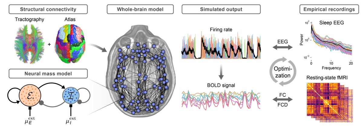
The figure below shows a schematic of how a brain network is constructed:
Examples:
Single node simulation ·
Whole-brain network ·
Parameter exploration ·
Evolutionary optimization
Whole-brain modeling
Typically, in whole-brain modeling, diffusion tensor imaging (DTI) is used to infer the structural connectivity (the connection strengths) between different brain areas. In a DTI scan, the direction of the diffusion of molecules is measured across the whole brain. Using tractography, this information can yield the distribution of axonal fibers in the brain that connect distant brain areas, called the connectome. Together with an atlas that divides the brain into distinct areas, a matrix can be computed that encodes how many fibers go from one area to another, the so-called structural connectivity (SC) matrix. This matrix defines the coupling strengths between brain areas and acts as an adjacency matrix of the brain network. The fiber length determines the signal transmission delay between all brain areas. Combining the structural data with a computational model of the neuronal activity of each brain area, we can create a dynamical model of the whole brain.
The resulting whole-brain model consists of interconnected brain areas, with each brain area having their internal neural dynamics. The neural activity can also be used to simulate hemodynamic BOLD activity using the Balloon-Windkessel model, which can be compared to empirical fMRI data. Often, BOLD activity is used to compute correlations of activity between brain areas, the so called resting state functional connectivity, resulting in a matrix with correlations between each brain area. This matrix can then be fitted to empirical fMRI recordings of the resting-state activity of the brain.
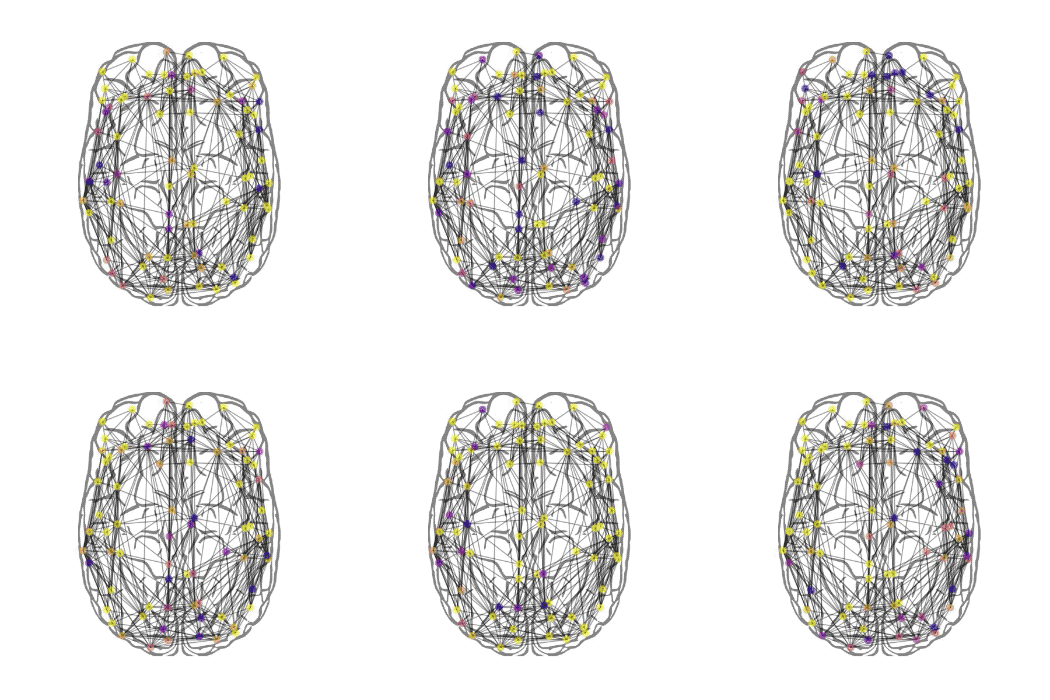
Below is an animation of the neuronal activity of a whole-brain model plotted on a brain.
Installation
The easiest way to get going is to install the pypi package using pip:
pip install neurolib
Alternatively, you can also clone this repository and install all dependencies with
git clone https://github.com/neurolib-dev/neurolib.git
cd neurolib/
pip install -r requirements.txt
pip install .
It is recommended to clone or fork the entire repository since it will also include all examples and tests.
Project layout
neurolib/	 				# Main module
├── models/ 					# Neural mass models
	├──model.py 				# Base model class
	└── /.../ 				# Implemented mass models
├── optimize/ 					# Optimization submodule
	├── evolution/ 				# Evolutionary optimization
	└── exploration/ 			# Parameter exploration
├── data/ 					# Empirical datasets (structural, functional)
├── utils/					# Utility belt
	├── atlases.py				# Atlases (Region names, coordinates)
	├── collections.py			# Custom data types
	├── functions.py 			# Useful functions
	├── loadData.py				# Dataset loader
	├── parameterSpace.py			# Parameter space
	├── saver.py 				# Save simulation outputs
	├── signal.py				# Signal processing functions
	└── stimulus.py 			# Stimulus construction
├── examples/					# Example Jupyter notebooks
├── docs/					# Documentation
└── tests/					# Automated tests
Examples
Example IPython Notebooks on how to use the library can be found in the ./examples/ directory, don't forget to check them out! You can run the examples in your browser using Binder by clicking here or one of the following links:
- Example 0.0 - Basic use of the
alnmodel - Example 0.3 - Fitz-Hugh Nagumo model
fhnon a brain network - Example 0.6 - Minimal example of how to implement your own model in
neurolib - Example 1.2 - Parameter exploration of a brain network and fitting to BOLD data
- Example 2.0 - A simple example of the evolutionary optimization framework
A basic overview of the functionality of neurolib is also given in the following.
Single node
This example is available in detail as a IPython Notebook.
To create a single aln model with the default parameters, simply run
from neurolib.models.aln import ALNModel

model = ALNModel()
model.params['sigma_ou'] = 0.1 # add some noise

model.run()
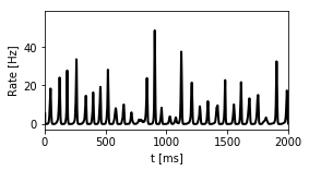
The results from this small simulation can be plotted easily:
import matplotlib.pyplot as plt
plt.plot(model.t, model.output.T)
Whole-brain network
A detailed example is available as a IPython Notebook.
To simulate a whole-brain network model, first we need to load a DTI and a resting-state fMRI dataset. neurolib already provides some example data for you:
from neurolib.utils.loadData import Dataset

ds = Dataset("gw")
The dataset that we just loaded, looks like this:

We initialize a model with the dataset and run it:
model = ALNModel(Cmat = ds.Cmat, Dmat = ds.Dmat)
model.params['duration'] = 5*60*1000 # in ms, simulates for 5 minutes

model.run(bold=True)
This can take several minutes to compute, since we are simulating 80 brain regions for 5 minutes realtime. Note that we specified bold=True which simulates the BOLD model in parallel to the neuronal model. The resulting firing rates and BOLD functional connectivity looks like this:
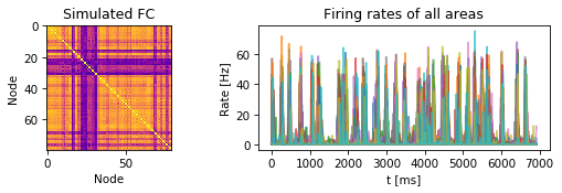
The quality of the fit of this simulation can be computed by correlating the simulated functional connectivity matrix above to the empirical resting-state functional connectivity for each subject of the dataset. This gives us an estimate of how well the model reproduces inter-areal BOLD correlations. As a rule of thumb, a value above 0.5 is considered good.
We can compute the quality of the fit of the simulated data using func.fc() which calculates a functional connectivity matrix of N (N = number of brain regions) time series. We use func.matrix_correlation() to compare this matrix to empirical data.
scores = [func.matrix_correlation(func.fc(model.BOLD.BOLD[:, 5:]), fcemp) for fcemp in ds.FCs]

print("Correlation per subject:", [f"{s:.2}" for s in scores])
print(f"Mean FC/FC correlation: {np.mean(scores):.2}")
Correlation per subject: ['0.34', '0.61', '0.54', '0.7', '0.54', '0.64', '0.69', '0.47', '0.59', '0.72', '0.58']
Mean FC/FC correlation: 0.58
Parameter exploration
A detailed example of a single-node exploration is available as a IPython Notebook. For an example of a brain network exploration, see this Notebook.
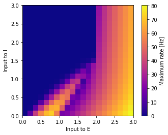
Whenever you work with a model, it is of great importance to know what kind of dynamics it exhibits given a certain set of parameters. It is often useful to get an overview of the state space of a given model of interest. For example in the case of aln, the dynamics depends a lot on the mean inputs to the excitatory and the inhibitory population. neurolib makes it very easy to quickly explore parameter spaces of a given model:
# create model
model = ALNModel()
# define the parameter space to explore
parameters = ParameterSpace({"mue_ext_mean": np.linspace(0, 3, 21),  # input to E
		"mui_ext_mean": np.linspace(0, 3, 21)}) # input to I

# define exploration
search = BoxSearch(model, parameters)

search.run()
That's it!. You can now use the builtin functions to load the simulation results from disk and perform your analysis:
search.loadResults()

# calculate maximum firing rate for each parameter
for i in search.dfResults.index:
    search.dfResults.loc[i, 'max_r'] = np.max(search.results[i]['rates_exc'][:, -int(1000/model.params['dt']):])
We can plot the results to get something close to a bifurcation diagram!
Evolutionary optimization
A detailed example is available as a IPython Notebook.
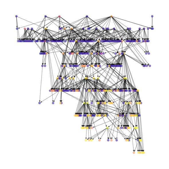
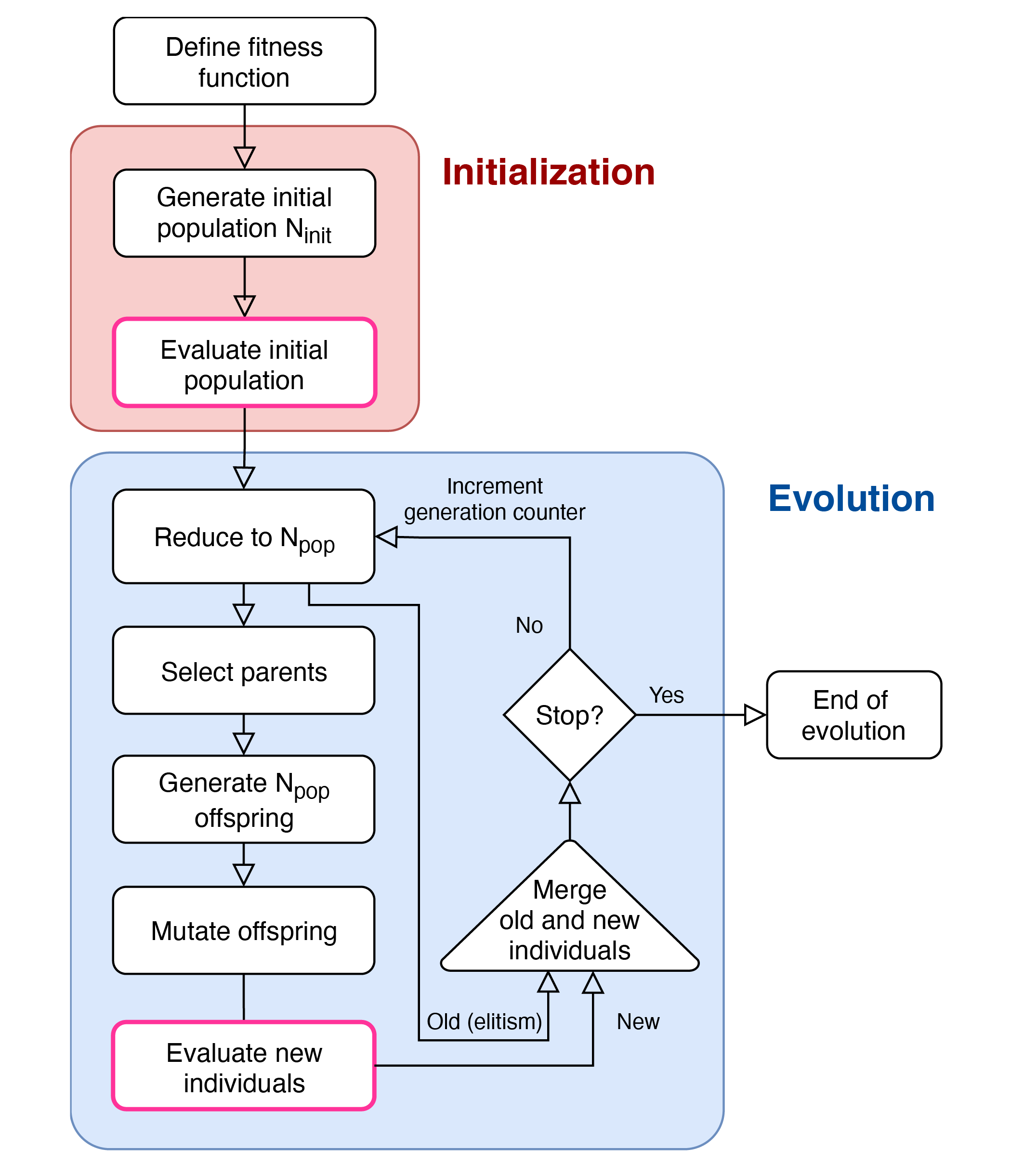
neurolib also implements evolutionary parameter optimization, which works particularly well with brain networks. In an evolutionary algorithm, each simulation is represented as an individual and the parameters of the simulation, for example coupling strengths or noise level values, are represented as the genes of each individual. An individual is a part of a population. In each generation, individuals are evaluated and ranked according to a fitness criterion. For whole-brain network simulations, this could be the fit of the simulated activity to empirical data. Then, individuals with a high fitness value are selected as parents and mate to create offspring. These offspring undergo random mutations of their genes. After all offspring are evaluated, the best individuals of the population are selected to transition into the next generation. This process goes on for a given amount generations until a stopping criterion is reached. This could be a predefined maximum number of generations or when a large enough population with high fitness values is found.
An example genealogy tree is shown below. You can see the evolution starting at the top and individuals reproducing generation by generation. The color indicates the fitness.
neurolib makes it very easy to set up your own evolutionary optimization and everything else is handled under the hood. You can chose between two implemented evolutionary algorithms: adaptive is a gaussian mutation and rank selection algorithm with adaptive step size that ensures convergence (a schematic is shown in the image below). nsga2 is an implementation of the popular multi-objective optimization algorithm by Deb et al. 2002.
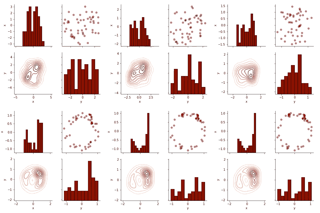
Of course, if you like, you can dig deeper, define your own selection, mutation and mating operators. In the following demonstration, we will simply evaluate the fitness of each individual as the distance to the unit circle. After a couple of generations of mating, mutating and selecting, only individuals who are close to the circle should survive:
from neurolib.utils.parameterSpace import ParameterSpace
from neurolib.optimize.evolution import Evolution

def optimize_me(traj):
    ind = evolution.getIndividualFromTraj(traj)

    # let's make a circle
    fitness_result = abs((ind.x**2 + ind.y**2) - 1)

    # gather results
    fitness_tuple = (fitness_result ,)
    result_dict = {"result" : [fitness_result]}

    return fitness_tuple, result_dict

# we define a parameter space and its boundaries
pars = ParameterSpace(['x', 'y'], [[-5.0, 5.0], [-5.0, 5.0]])

# initialize the evolution and go
evolution = Evolution(optimize_me, pars, weightList = [-1.0], POP_INIT_SIZE= 100, POP_SIZE = 50, NGEN=10)
evolution.run()
That's it! Now we can check the results:
evolution.loadResults()
evolution.info(plot=True)
This will gives us a summary of the last generation and plots a distribution of the individuals (and their parameters). Below is an animation of 10 generations of the evolutionary process. Ass you can see, after a couple of generations, all remaining individuals lie very close to the unit circle.
More information
Built With
neurolib is built using other amazing open source projects:
- pypet - Python parameter exploration toolbox
- deap - Distributed Evolutionary Algorithms in Python
- numpy - The fundamental package for scientific computing with Python
- numba - NumPy aware dynamic Python compiler using LLVM
- Jupyter - Jupyter Interactive Notebook
How to cite
Cakan, C., Jajcay, N. & Obermayer, K. neurolib: A Simulation Framework for Whole-Brain Neural Mass Modeling. Cogn. Comput. (2021). https://doi.org/10.1007/s12559-021-09931-9
@article{cakan2021,
    author={Cakan, Caglar and Jajcay, Nikola and Obermayer, Klaus},
    title={neurolib: A Simulation Framework for Whole-Brain Neural Mass Modeling},
    journal={Cognitive Computation},
    year={2021},
    month={Oct},
    issn={1866-9964},
    doi={10.1007/s12559-021-09931-9},
    url={https://doi.org/10.1007/s12559-021-09931-9}
}
Get in touch
Caglar Cakan (cakan@ni.tu-berlin.de)
Department of Software Engineering and Theoretical Computer Science, Technische Universität Berlin, Germany
Bernstein Center for Computational Neuroscience Berlin, Germany
Acknowledgments
This work was supported by the Deutsche Forschungsgemeinschaft (DFG, German Research Foundation) with the project number 327654276 (SFB 1315) and the Research Training Group GRK1589/2.
Project details
Release history Release notifications | RSS feed
Download files
Download the file for your platform. If you're not sure which to choose, learn more about installing packages.
Source Distribution
Built Distribution
Filter files by name, interpreter, ABI, and platform.
If you're not sure about the file name format, learn more about wheel file names.
Copy a direct link to the current filters
File details
Details for the file neurolib-0.6.2.tar.gz.
File metadata
- Download URL: neurolib-0.6.2.tar.gz
- Upload date:
- Size: 8.3 MB
- Tags: Source
- Uploaded using Trusted Publishing? No
- Uploaded via: twine/4.0.1 CPython/3.7.13
File hashes
| Algorithm | Hash digest | |
|---|---|---|
| SHA256 |
d2eb02e1096928896e3735577cb170df94c8059b549ef022e924f3b8fa50c691
|
|
| MD5 |
5c1447df616018480c8c7aa424db1736
|
|
| BLAKE2b-256 |
e117b5cf2c5279a4cf6e8c8382dbe98e6951b08c2ae3daa0e89b1dc912811537
|
File details
Details for the file neurolib-0.6.2-py3-none-any.whl.
File metadata
- Download URL: neurolib-0.6.2-py3-none-any.whl
- Upload date:
- Size: 8.3 MB
- Tags: Python 3
- Uploaded using Trusted Publishing? No
- Uploaded via: twine/4.0.1 CPython/3.7.13
File hashes
| Algorithm | Hash digest | |
|---|---|---|
| SHA256 |
0e2528dbb08e8ebac66e633660f6a8e5cd51b7b7de0ab76b4f1a397496ca8896
|
|
| MD5 |
9a6eb410f2f71569a5041466b04e50bb
|
|
| BLAKE2b-256 |
744f0ee159bd82c77bbfc236f649506a146d44d61b9711f534e036dcd75c22f5
|


