Antenna plotting program for plotting antenna simulation results

Project description
This is a program to plot antenna-related data resulting from an antenna simulation. It can read the text output produced by nec2c, my python mininec port pymininec, output from the original Basic implementations of Mininec, ASAP, and with a separate command-line tool the output of 3D antenna pattern from EZNEC.
Most notably it can plot antenna far-field pattern in both 2D (Azimuth and Elevation) and 3D (as a 3D graphic that can be rotated and zoomed). It supports a local display program (using matplotlib) and a HTML output version that displays everything using javascript (using plotly). The program features a --help option.
The program started out as a companion-program to my pymininec project and is now an independent program.
The plot program can also display output files of nec2c, ASAP, and EZNEC, not only from pymininec.
Standalone Plotting with Matplotlib
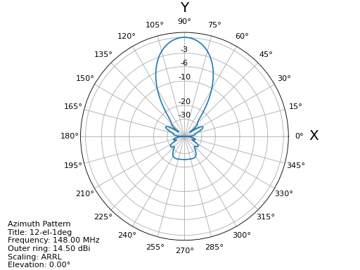
The default is to plot all available graphics, including an interactive 3d view. In addition with the --azimuth or --elevation options you can get an Azimuth diagram:
plot-antenna --azimuth test/12-el-1deg.pout
or an elevation diagram:
plot-antenna --elevation test/12-el-1deg.pout
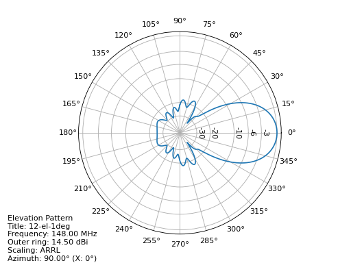
respectively. Note that I used an output file with 1-degree resolution in elevation and azimuth angles not with 5 degrees as in the example above. The pattern look smoother but a 3D-view in matplotlib will be very slow due to the large number of points. This problem does not occur when using the plotly backend.
Sometimes we do not want the azimuth plot at the maximum elevation angle or the elevation plot at the maximum azimuth angle. You can specify the elevation angle for the azimuth plot with the --angle-elevation option and the azimuth angle for the elevation plot with --angle-azimuth. An example azimuth plot of the same antenna at an elevation angle of 15° can be plotted with:
plot-antenna --azimuth --angle-elevation=15 test/12-el-1deg.pout
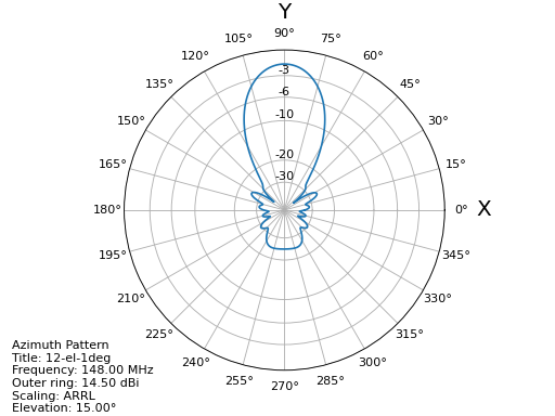
As you can see, the azimuth-plot is scaled to the maximum gain of the antenna. Sometimes we want to scale the gain to the maximum at that elevation (or azimuth) angle. This can be achieved with the --scale-by-angle option:
plot-antenna --azi --angle-ele=15 --scale-by-angle test/12-el-1deg.pout
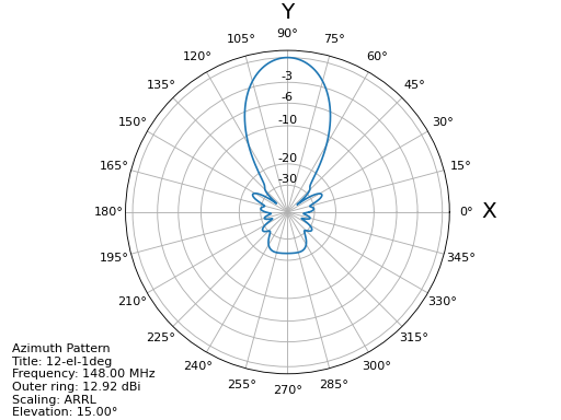
You can see that now the pattern is scaled to the maximum at that elevation angle. The outer ring now has 12.92 dBi instead of 14.50 dBi.
The plot program also has a --help option for further information. In particular the scaling of the antenna plot can be selected using the --scaling-method option with an additional keyword which can be one of linear, linear_db, and linear_voltage in addition to the default of arrl scaling. You may consult Cebik’s [1] article for explanation of the different diagrams. The linear_voltage option is not explained by Cebik, it is in-between the linear and linear_db scaling options.
The latest version accepts several plot parameters, --elevation, --azimuth, --plot3d, --plot-vswr, and --geo which are plotted into one diagram. The default is to plot the first four graphs. With the --output option pictures can directly be saved without displaying the graphics on the screen. Note that unfortunately the geometry display with the --geo option does not perform very well because matplotlib has poor support for panning and scaling in 3D plots. It works fine with the plotly backend.
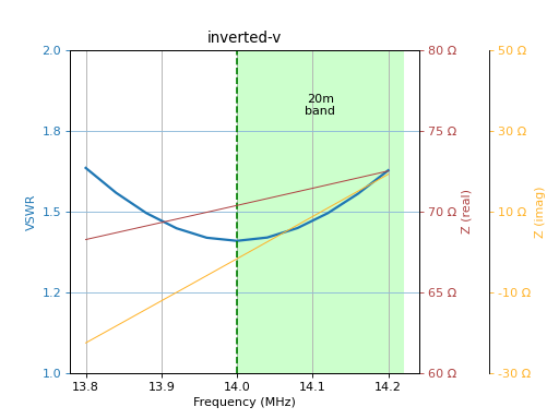
There are sub-options that change the behavior of the main option. For the SWR plot, coloring of Ham-Radio bands and the display of the antenna impedance can be turned on with --swr-show-bands and --swr-show-impedance, respectively. An example may look like the following:
The latest version has key-bindings for scrolling through the frequencies of an antenna simulation. These keybindings only work for the matplotlib backend. If you have an output file with a simulation of multiple frequencies you can display diagrams for the next frequency by typing +, and to the previous frequency by typing -. For newer versions of matplotlib you can display a scrollbar for the frequencies with the --with-slider option.
Other keybindings switch the scaling for the antenna plots, a switches to arrl scaling, l switches to linear scaling, d switches to linear dB scaling, and v switches to linear voltage scaling.
Finally the w key toggles display of the 3d diagram from/to wireframe display. Note that the wireframe display may not be supported on all versions of matplotlib and/or graphics cards.
Plotting for the Browser with Plotly
All the plot supported for matplotlib are also supported with plotly. These are --elevation, --azimuth, --plot3d, --plot-vswr, and --geo. The plots can be either exported to a .html file using the -H or --export-html option (with an additional filename to export to) or injected into a running browser using the -S or --show-in-browser option.
Unlike for matplotlib, each plot selected with an option is either shown in a separate window in the browser or exported to a separate file. If exporting to a file, additional output options can be selected with the --html-export-option setting. The default is to export the file with all javascript included (adds about 3MB to the file size). With --html-export-option=directory the javascript is not included and a plotly.min.js file is expected in the same directory as the exported file. This file ships with the plotly distribution. When exporting to a file, the plot name is appended to the file name given, this allows export to several different plots in one program invocation.
The scaling variants selected with the --scaling-method option cannot currently be changed at runtime with the plotly plots. As with matplotlib, the default is arrl scaling. When using scaling in dB, the minimum dB value can be specified with the --scaling-mindb option.
Like with matplotlib there are sub-options that change the behavior of the main option. For the SWR plot, coloring of Ham-Radio bands and the display of the antenna impedance can be turned on with --swr-show-bands and --swr-show-impedance, respectively
All plots are interactive. For the far-field pattern plots (Azimuth, Elevation, 3D) frequencies can be selected in the legend to the right of the plot. With mouse-over you can see the current angle (Elevation or Azimuth with the 2D plots and both for the 3D plot) and the gain at that point. For the 2D variants, more than one frequency can be selected for plotting. This allows comparison of pattern between different frequencies. For the 3D plot, the frequencies in the legend act like radio-buttons, only one at a time can be selected.
With the --geo option you get a display of the antenna geometry. Unfortunately plotly seems to have limitations on the zoom depths, so for large antennas it is not possible to see the plot in deep detail. As of this writing not all geometry details are displayed. In particular 2D patches in NEC and transmission lines in NEC are not shown.
Input Sources
As already mentioned previously, plot-antenna can take input produced by a couple of antenna simulation tools. Originally written for my re-implementation of Mininec, pymininec, it can also use the output from the original Mininec written in Basic, from nec2c, and from the Antenna Scatterers Analysis Program ASAP. It automatically detects in which format the input is and acts accordingly.
In addition there is a separate command-line tool, plot-eznec that can be used to visualize the output from EZNEC’s export function.
It has also been used for visualizing antenna measurement data. An example from a contributed measurement is here:
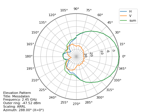
Note that for the measurement-data the unit of the data is not in dBi but (because it was measured and not calibrated to dBi) in dBm. The measurements were separate for horizontal and vertical polarization.
The program for plotting the measurements is in plot_antenna/contrib.py. It can serve as an example of how to plot your own data with plot-antenna. The eznec program in plot_antenna/eznec.py might even be better in this regard. See the next section on documentation of the plot-antenna API.
Running the Tests
For running the plotly tests, the kaleido python package needs to be installed. For Debian Trixie and earlier version 0.2.1 is needed. This is installed with pip as shown below, if you don’t want to mess with the --break-system-packages option, installing everything into a virtual environment is the way to go:
python3 -m pip install kaleido==0.2.1 --break-system-packages
The tests use pictures saved in test/pics and will compare – depending on matplotlib or plotly version – the picture matching the backend version to the picture produced during the test. For this to work, especially for plotly, the correct fonts need to be installed. Plotly seems to prefer the Open Sans font family. So at least on Debian the package fonts-open-sans needs to be installed. Otherwise the tests fail because the pictures do not match. If a test fails a picture with the extension .debug will be produced in the directory test/pics. If differences are not immediately visible, the compare program from imagemagick may help.
Plot-Antenna API
The main class to plot things is the Gain_Plot class. It gets the command-line arguments and the gain data to plot. Note that the class is a little mis-named now because it can also do all the other plots (e.g. standing wave ratio, SWR). The gain data passed to the constructor of Gain_Plot gets a dictionary of Gain_Data objects. The keys of the dictionary are tuples (frequency, string) where the frequency is the frequency of the Gain_Data and the string is used for describing what is plotted. Since plot-antenna can have traces for the different polarizations in the same plot, usually the string is one of H for horizontal polarization, V for vertical polarization and sum for the sum of all polarizations. Of course only the sum can be provided if we do not want multiple polarizations.
If you are not plotting gain but, say, only SWR data, the gain data object passed to the Gain_Plot constructor may be None.
The Gain_Data object gets a list of frequencies in the constructor. It has an internal pattern dictionary which stores the gain values by a tuple of (theta, phi) where theta is the elevation angle (measured from the zenith=0 degrees) and the azimuth angle phi measured from the positive X-axis. The gain values in this data structure are in dBi (Decibel over an isotropic radiator).
A simple program to construct an azimuth plot of an antenna that has the same pattern in all directions (gain=0dB) would be:
import numpy as np
from plot_antenna import plot_antenna

# Compute args, see below
frequency = 430.0
polarization = 'sum'
key = (frequency, polarization)
gdict = {key: plot_antenna.Gain_Data (key)}
data = gdict [key].pattern
for theta in np.arange (0, 181, 10):
    for phi in np.arange (0, 361, 10):
        data [(theta, phi)] = 0.0
gp = plot_antenna.Gain_Plot (args, gdict)
gp.compute ()
gp.plot ()
In the latest version you can also directly pass numpy arrays for gain, theta, and phi angles, angles are in degrees:
import numpy as np
from plot_antenna import plot_antenna

# Compute args, see below
frequency = 430.0
polarization = 'sum'
key = (frequency, polarization)
thetas = np.arange (0, 181, 10)
phis   = np.arange (0, 361, 10)
gains  = np.zeros ((19, 37))
gdict  = {key: plot_antenna.Gain_Data.from_gains (key, gains, thetas, phis)}
gp = plot_antenna.Gain_Plot (args, gdict)
gp.compute ()
gp.plot ()
The parsed arguments can typically be constructed by calling one of the argument parsing functions. These need not be given the real command line arguments but can be called with an empty string list, e.g.:
# Initialize command options with general options
cmd = plot_antenna.options_general ()
# Add gain options
plot_antenna.options_gain (cmd)
# Parse empty arguments resulting in default args
args = plot_antenna.process_args (cmd, [])
# The filename is needed internally for computing default title
args.filename = ''
# Title
args.title = 'My Title'
# We might want to ship result to running browser with plotly
# args.show_in_browser = True
# If we want to do a 3d-plot we set args.plot3d, we could also set
# args.azimuth to get an azimuth plot. Both variables can be set and
# we get both plots (one after the other with matplotlib, both in
# different browser windows with plotly)
args.azimuth = False
args.plot3d  = True
The cmd variable is a python ArgumentParser object. So if you are parsing command line arguments you can add your own options before calling process_args.
If not parsing argument from the command line and arguments should be changed this can be done by directly modifying args, e.g.:
args.title = 'This is the title of my plot'
A full but short implementation of a usage of this API can be found in the companion program for reading EZNEC data in plot_antenna/eznec.py. This example can be found in example.py.
Release Notes
v2.4: Bug-fixes, coordinate transformation
Fix max theta gain computation: We need to take both sides of phi into account
Allow to directly pass numpy arrays in API
Coordinate transform for a contributed setup for a measurement device
Update tests for debian trixie, in particular use better font defaults that are more likely to be the same on multiple architectures
v2.3: Fix nec geo computation
Fix a bug when parsing NEC geo info, in particular back-references in geometry segments
Update tests for recent changes, unfortunately the plotly PNG pics seem not to be reproduceable across different installations of the same plotly version
v2.2: Fix radial axis range of polar plots
Polar plots were scaled differently depending on data, we now force the polar axis range to a maximum of 1.01 (on both, matplotlib and plotly backends) so that the trace(s) always fit without truncating the trace at the boundary
v2.1: Scale by angle
New option --scale-by-angle that allows to scale the azimuth or elevation pattern to the maximum at the current elevation- or azimuth angle instead of the global maximum, thanks to Daniel Bruschinski for suggesting this
Add a little documentation how to use the API, thanks to Alex, VE3NEA for suggesting this in a github issue.
v2.0: More input formats
Import from EZNEC exported pattern data
Import from the Antenna Scatterers Analysis Program ASAP
Import from ancient Mininec versions written in Basic
Add a --maxgain option to normalize the gain of the outer ring
Display polarization for plotly when the single polarization is not “sum”.
Title added for geo, 3d, and swr plots
Add more tests
Tests: Now use explicitly-stored pictures instead of only picture hashes: It is much easier if we can compare the produced picture to the expected picture.
Numerous bug-fixes
v1.8: Allow plotting of measurement data
Deal with sparse matrix for plot values
Interpolation of measured values in Phi (Azimuth) direction
Add STL output of 3d pattern with optional library
Allow setting the dB-unit (e.g. dBm for measurements)
Allow plotting by polarization
Version computation changed to allow install from git url
Note: Smith chart with matplotlib currently needs my patched pySmithPlot library. You can install this with:
python -m pip install pysmithplot@git+https://github.com/schlatterbeck/pySmithPlot.git
v1.7: Add Smith charts, optionally show impedance and band in VSWR plots
Many of the changes in this and several previous versions were suggested by Rob Banfield, DM1CM: Adding the bands and impedance to the VSWR plot are his idea as well as adding a Smith chart. Due to his attention to detail this release corrects a lot of rough edges of previous versions. Thanks Rob!
The aspect ratio in 3D plotly plots is now correct. It used to be a little too wide in the X direction
Add Smith chart display
Options to add the impedance (either as real/imag or |Z|/phi (Z)) in the VSWR plot
Option to show the ham radio bands in the VSWR plot
Show loads and excitation(s) in geo plot, add ground to geo plot
Margin of 3D plots in plotly are much wider now by default and can be configured with an option
The style how the gain is displayed in the plotly 3D color bar can now be configured to save space (either relative or absolute gain in dB or dBi, the default is both)
When there is only one frequency in the 3D plot, remove the frequency legend
Add LICENSE file and pyproject.toml for newer install mechanisms in python
Add tests for plotly output
Use ppm images for the tests, the previously-used png images did contain the matplotlib version and thus were different for each version – the ppm images do not have that problem, there are still many differences with different matplotlib versions
v1.6: More SWR plot changes
Make SWR-plot vertical line colors configurable
Rename elevation-angle and azimuth-angle options to angle-elevation and angle-azimuth so that we can again request an elevation/azimuth plot with shortened options like --ele or --azi
Sort options lexicographically on --help
v1.5: Allow target SWR frequency in VSWR plot
Add command-line option --target-swr-frequency
Draw user-specifed target frequency in red, best (minimum) swr in grey
v1.4: Reset button and VSWR-Plot improvements
Add grid and minimum-SWR vertical line to VSWR plot
Remove display of frequency in mouse-over (in polar plots and 3D plot)
Make polar reset button reset more parameters
v1.3: Add a reset button to plotly polar plots
The polar plots, when zoomed in, could only be reset to the unzoomed view with a double-click. All other plots do have a reset button, add one for the polar plots, too.
v1.2: Allow specification of title (legend) font size in plotly version
For some application (e.g. when using the plotly graphics inside a html iframe) the title (or we may want to call it legend) of the graphics may collide with the graphics itself. We can now specify the font size with --title-font-size. This option currently works only with plotly graphics.
v1.1: Specification of azimuth / elevation angle
Now we can specify an azimuth angle for elevation plot and an elevation angle for azimuth plots.
Bug-fix in computation of maximum gain azimuth direction: If the maximum gain in theta direction goes up or down, the azimuth angle would be computed incorrectly because all gain values at that theta angle are the same for all azimuth angles.
Sort options: Since there are some options that only exist when some packages are installed we sort options instead of trying to add them in the correct order.
v1.0: Initial Release
Release history Release notifications | RSS feed


Download files
Download the file for your platform. If you're not sure which to choose, learn more about installing packages.
Source Distribution
Built Distribution
Filter files by name, interpreter, ABI, and platform.
If you're not sure about the file name format, learn more about wheel file names.
Copy a direct link to the current filters
File details
Details for the file plot_antenna-2.4.tar.gz.
File metadata
- Download URL: plot_antenna-2.4.tar.gz
- Upload date:
- Size: 52.4 kB
- Tags: Source
- Uploaded using Trusted Publishing? No
- Uploaded via: twine/6.1.0 CPython/3.13.5
File hashes
| Algorithm | Hash digest | |
|---|---|---|
| SHA256 |
bde9976fe48c825fbed152131b9bda5700f7bc52f1e401ed00931d8293cd7720
|
|
| MD5 |
1f43c6a78d639a50e92e10bcd484d542
|
|
| BLAKE2b-256 |
3b751e888045bf68991e677a2b91e10a5c0a6f5aeb365bbb6bbad2efdc6e1802
|
File details
Details for the file plot_antenna-2.4-py3-none-any.whl.
File metadata
- Download URL: plot_antenna-2.4-py3-none-any.whl
- Upload date:
- Size: 40.5 kB
- Tags: Python 3
- Uploaded using Trusted Publishing? No
- Uploaded via: twine/6.1.0 CPython/3.13.5
File hashes
| Algorithm | Hash digest | |
|---|---|---|
| SHA256 |
987d8cbebdbe2aee73eddecc811e6d8a488bff757e14076b5e2ee3ef715dbff0
|
|
| MD5 |
3c707b6ce1254d8efd7f932d883c37a4
|
|
| BLAKE2b-256 |
fe38b4496650bfd5221b5621c76bf4c15302dce1c3379fb1fb34bc07b961e3dc
|


