Package to compute Bayesian posterior distribution for transversal velocity using parallaxes and proper motions.

Project description
post-velocity
Package to compute Bayesian posterior distribution for transversal velocity using parallaxes and proper motions. Code is designed for the cases when the parallax uncertainty is significant while proper motion is measured with greater precision.
Introduction
The transversal velocities of stars are important in many astrophysical applications such as a search for run-away stars and ultra-high velocity white dwarfs. These velocities are often computed using measured parallaxes and proper motions of stars. The parallax measurements are often have limited accuracy especially for distances of a few kpc.
Installation
The package is available at pypi so it can be installed using pip:
pip install post_velocity
Examples of the usage are available in folder examples.
Simple usage
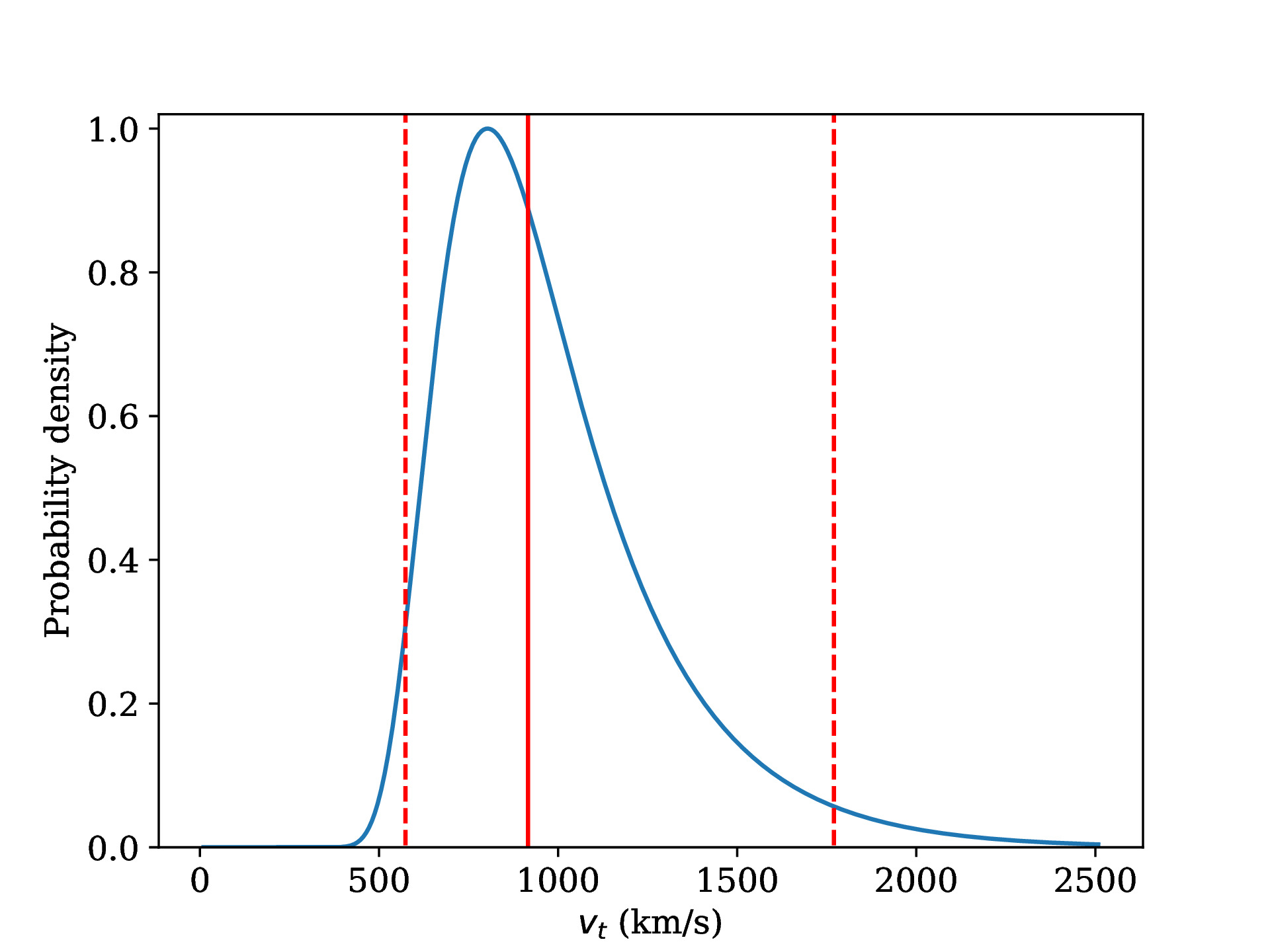
A simple example can be found in example.py. In this code I use parallax and proper motion measurements for Gaia DR3 5703888058542880896. Parallax is given in milliarcseconds and proper motion is in milliarcseconds per year.
from post_velocity import post_velocity
from math import *
import matplotlib.pyplot as plt

parallax = 1.3616973828503283
parallax_error = 0.31826717
pmra = 70.22832802893967
pmra_error = 0.31611034
pmdec = -195.65413513344822
pmdec_error = 0.2825489
l = radians(245.99334300224004)
b = radians(13.599432251899845)

meas = pmra, pmra_error, pmdec, pmdec_error, parallax, parallax_error, l, b
vtl, pvtl, idx025, idx50, idx975 = post_velocity.compute_posterior (meas)

plt.plot (vtl, pvtl)
plt.plot ([vtl[idx025], vtl[idx025]], [-0.5,1.1], 'r--')
plt.plot ([vtl[idx50],  vtl[idx50]],  [-0.5,1.1], 'r-')
plt.plot ([vtl[idx975], vtl[idx975]], [-0.5,1.1], 'r--')

plt.xlabel(r'$v_t$ (km/s)')
plt.ylabel(r'Probability density')
plt.ylim([0,1.02])
plt.savefig ('posterior_vt.pdf')
plt.show()
This code produces the following image. The red dashed lines show the five percent credible interval. The red solid line shows median of the posterior distribution.
Varying parameters of priors
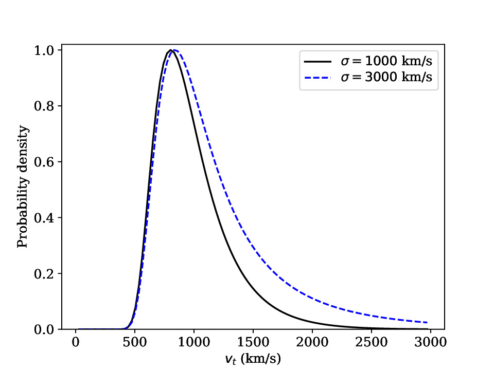
The basic function compute_posterior (meas, Rsun = 8.34, hz = 0.33, hr = 1.70, min_vt = 10, max_vt = 2500, n_step = 100, sigma = 1000) allows varying parameters of all priors involved in the calculations. Below I show how to change parameters of the velocity prior:
from post_velocity import post_velocity
from math import *
import matplotlib.pyplot as plt

parallax = 1.3616973828503283   ## mas
parallax_error = 0.31826717     ## mas
pmra = 70.22832802893967        ## mas/year
pmra_error = 0.31611034         ## mas/year
pmdec = -195.65413513344822     ## mas/year
pmdec_error = 0.2825489         ## mas/year
l = radians(245.99334300224004) ## degrees to be converted to radians while working with the package
b = radians(13.599432251899845) ## degrees to be converted to radians while working with the package

meas = pmra, pmra_error, pmdec, pmdec_error, parallax, parallax_error, l, b

## Posterior will be computed for the velocity range from min_vt to max_vt
min_vt = 30   ## km/s
max_vt = 3000 ## km/s

## Vary velocity prior
sigma1000 = 1000.0 ## km/s
sigma3000 = 3000.0 ## km/s

vtl1, pvtl1, idx025, idx50, idx975 = post_velocity.compute_posterior (meas, min_vt=min_vt, max_vt=max_vt, sigma=sigma1000)
vtl3, pvtl3, idx025, idx50, idx975 = post_velocity.compute_posterior (meas, min_vt=min_vt, max_vt=max_vt, sigma=sigma3000)

plt.plot (vtl1, pvtl1, 'k-', label=r'$\sigma=1000$ km/s')
plt.plot (vtl3, pvtl3, 'b--', label=r'$\sigma=3000$ km/s')

plt.xlabel(r'$v_t$ (km/s)')
plt.ylabel(r'Probability density')
plt.ylim([0,1.02])
plt.legend()
plt.savefig ('posterior_vt_sigma.pdf')
plt.show()
We show the result below.
Advanced usage
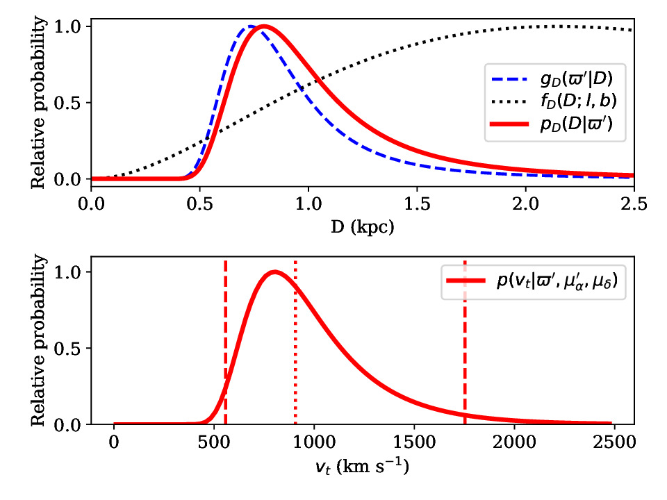
The package also provide functions fD (D, gl, gb, hz, hr, Rsun) and g (D, varpi, sigma_varpi) which can be used to compute posterior for distances only.
from post_velocity import post_velocity
from math import *
import matplotlib.pyplot as plt
import numpy as np

parallax = 1.3616973828503283   ## mas
parallax_error = 0.31826717     ## mas
pmra = 70.22832802893967        ## mas/year
pmra_error = 0.31611034         ## mas/year
pmdec = -195.65413513344822     ## mas/year
pmdec_error = 0.2825489         ## mas/year
l = radians(245.99334300224004) ## degrees to be converted to radians while working with the package
b = radians(13.599432251899845) ## degrees to be converted to radians while working with the package

### Setting parameters of the Galactic prior

hz = 0.33   ## kpc
hr = 1.70   ## kpc
Rsun = 8.34 ## kpc

meas = pmra, pmra_error, pmdec, pmdec_error, parallax, parallax_error, l, b

vtl, pvtl, idx025, idx50, idx975 = post_velocity.compute_posterior (meas, Rsun = Rsun, hz = hz, hr = hr)


varpi = parallax
sigma_varpi = parallax_error

dl = []  ## array to keep distances
ggl = [] ## array to keep conditional probability to measure parallax if distances is fixed
ffl = [] ## array to keep Galactic prior


for k in range (1, 10000):

    d = 0.001 * k

    dl.append (d)
    ggl.append (post_velocity.g (d, varpi, sigma_varpi))  ##
    ffl.append (post_velocity.fD (d, l, b, hz, hr, Rsun)) ## Galactic prior for distances

ggl = np.asarray(ggl) / np.max(ggl)
ffl = np.asarray(ffl) / np.max(ffl)

tt = ggl*ffl ## here we compute posterior for distances
tt = tt / np.max(tt)

fig, axs = plt.subplots(2)

axs[0].plot (dl, ggl, '--', color='blue', label=r"$g_D (\varpi' | D)$", linewidth=2)
axs[0].plot (dl, ffl, ':', color='black', label=r'$f_D (D; l, b)$', linewidth=2)
axs[0].plot (dl, tt, '-', color='red', label=r"$p_D (D | \varpi')$", linewidth=3)
axs[0].set_xlim([0, 2.5])
axs[0].set_xlabel('D (kpc)')
axs[0].set_ylabel('Relative probability')
axs[0].legend()

axs[1].plot ([vtl[idx025], vtl[idx025]], [-1,1.5], '--', color='red', linewidth=2)
axs[1].plot ([vtl[idx50],  vtl[idx50]], [-1,1.5], ':',   color='red', linewidth=2)
axs[1].plot ([vtl[idx975], vtl[idx975]], [-1,1.5], '--', color='red', linewidth=2)

axs[1].plot (vtl, pvtl, color='red', linewidth=3, label=r"$p(v_t | \varpi', \mu_\alpha', \mu_\delta )$")

axs[1].set_xlabel(r'$v_t$ (km s$^{-1}$)')
axs[1].set_ylabel('Relative probability')
axs[1].set_ylim([0.0, 1.1])
axs[1].legend()
plt.tight_layout()
plt.savefig ('posterior_distance_vt.pdf')
plt.show()
This script produces the following image.
References
Details of the calculations can be found in two articles:
Igoshev, Verbunt & Cator (2016) A&A, 591, A123, 10
Igoshev, Perets & Hallakoun (2022) ArXiv: 2209.09915
Release history Release notifications | RSS feed

Download files
Download the file for your platform. If you're not sure which to choose, learn more about installing packages.
Source Distribution
Built Distribution
Filter files by name, interpreter, ABI, and platform.
If you're not sure about the file name format, learn more about wheel file names.
Copy a direct link to the current filters
File details
Details for the file post_velocity-0.1.2.tar.gz.
File metadata
- Download URL: post_velocity-0.1.2.tar.gz
- Upload date:
- Size: 17.5 kB
- Tags: Source
- Uploaded using Trusted Publishing? No
- Uploaded via: twine/4.0.1 CPython/3.7.6
File hashes
| Algorithm | Hash digest | |
|---|---|---|
| SHA256 |
1f06e3eb5d9eed90d8421fdb7f0cc5b45e979f925df63f61159b84040b262fcd
|
|
| MD5 |
63186640b71ab8e3bc30c7ac48117030
|
|
| BLAKE2b-256 |
6052a4b7e16f346e083cde64bde8125f91121a1493f287e0a8939dd4321609da
|
File details
Details for the file post_velocity-0.1.2-py3-none-any.whl.
File metadata
- Download URL: post_velocity-0.1.2-py3-none-any.whl
- Upload date:
- Size: 18.2 kB
- Tags: Python 3
- Uploaded using Trusted Publishing? No
- Uploaded via: twine/4.0.1 CPython/3.7.6
File hashes
| Algorithm | Hash digest | |
|---|---|---|
| SHA256 |
2fdd4800f285ce9022ea4ae8d26cb4c1a063e81223ab9e7063e6293c30d11f70
|
|
| MD5 |
cdb51d82e5be8536a2f5614cf09e9133
|
|
| BLAKE2b-256 |
a7e74f5c41c13deeb61f87fa8193c42febff32f13912f140a4c4da4c0d0c4d03
|


