
- primordial:
inflationary equation solver
- Version:
- 0.0.13
- Homepage:
- Documentation:





Description
primordial is a python package for solving cosmological inflationary equations.
It is very much in beta stage, and currently being built for research purposes.
Example Usage
Plot Background evolution
import numpy
import matplotlib.pyplot as plt
from primordial.solver import solve
from primordial.equations.inflation_potentials import ChaoticPotential
from primordial.equations.t.inflation import Equations, KD_initial_conditions
from primordial.equations.events import Inflation, Collapse

fig, ax = plt.subplots(3,sharex=True)
for K in [-1, 0, +1]:
     m = 1
     V = ChaoticPotential(m)
     equations = Equations(K, V)

     events= [Inflation(equations),                    # Record inflation entry and exit
              Inflation(equations, -1, terminal=True), # Stop on inflation exit
              Collapse(equations, terminal=True)]      # Stop if universe stops expanding

     N_p = -1.5
     phi_p = 23
     t_p = 1e-5
     ic = KD_initial_conditions(t_p, N_p, phi_p)
     t = numpy.logspace(-5,10,1e6)

     sol = solve(equations, ic, t_eval=t, events=events)

     ax[0].plot(sol.N(t),sol.phi(t))
     ax[0].set_ylabel(r'$\phi$')

     ax[1].plot(sol.N(t),sol.H(t))
     ax[1].set_yscale('log')
     ax[1].set_ylabel(r'$H$')

     ax[2].plot(sol.N(t),1/(sol.H(t)*numpy.exp(sol.N(t))))
     ax[2].set_yscale('log')
     ax[2].set_ylabel(r'$1/aH$')

ax[-1].set_xlabel('$N$')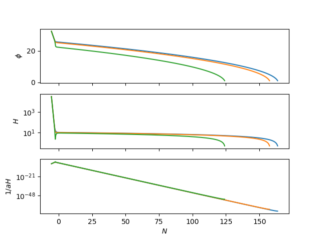
Plot mode function evolution
import numpy
import matplotlib.pyplot as plt
from primordial.solver import solve
from primordial.equations.inflation_potentials import ChaoticPotential
from primordial.equations.t.mukhanov_sasaki import Equations, KD_initial_conditions
from primordial.equations.events import Inflation, Collapse, ModeExit

fig, axes = plt.subplots(3,sharex=True)
for ax, K in zip(axes, [-1, 0, +1]):
    ax2 = ax.twinx()
    m = 1
    V = ChaoticPotential(m)
    k = 100
    equations = Equations(K, V, k)

    events= [
            Inflation(equations),                    # Record inflation entry and exit
            Collapse(equations, terminal=True),      # Stop if universe stops expanding
            ModeExit(equations, +1, terminal=True, value=1e1*k)   # Stop on mode exit
            ]


    N_p = -1.5
    phi_p = 23
    t_p = 1e-5
    ic = KD_initial_conditions(t_p, N_p, phi_p)
    t = numpy.logspace(-5,10,1e6)

    sol = solve(equations, ic, t_eval=t, events=events)

    N = sol.N(t)
    ax.plot(N,sol.R1(t), 'k-')
    ax2.plot(N,-numpy.log(sol.H(t))-N, 'b-')

    ax.set_ylabel('$\mathcal{R}$')
    ax2.set_ylabel('$-\log aH$')

    ax.text(0.9, 0.9, r'$K=%i$' % K, transform=ax.transAxes)

axes[-1].set_xlabel('$N$')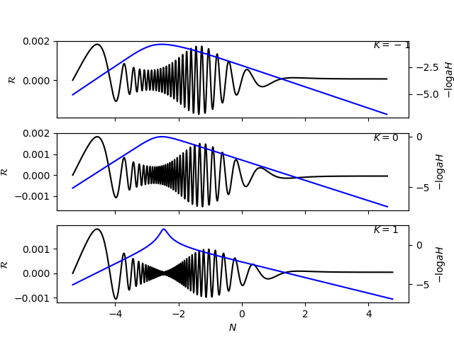
To do list
Eventually would like to submit this to JOSS. Here are things to do before then:
Cosmology
Slow roll initial conditions
Mukhanov Sazaki evolution in \(N\)
add \(\eta\) as independent variable
add \(\phi\) as independent variable
Code
Documentation
- Tests
100% coverage
interpolation
cosmology
1 maintainer

Metadata
1 maintainer
Release files for primordial 0.0.13
For a detailed explanation of source distributions (sdists) and built distributions (wheels), please see the package formats documentation.
Source distribution (sdist)
| File | Size | Uploaded | |
|---|---|---|---|
| primordial-0.0.13.tar.gz | 9.8 kB | Details |
Release files / primordial-0.0.13.tar.gz
| Download URL | primordial-0.0.13.tar.gz |
|---|---|
| Size | 9.8 kB |
| Tags | Source |
|
SHA-256 checksum How to use checksums |
0d6a573e8f76bc2f52a6c6a40c95534746bd23b6de2b1c4ded6cbbbf944e2e88
|
|
BLAKE2b-256 checksum How to use checksums |
0d31a2b6265a5ff9104510ed0dc692d77d24c8bb3f1332700a08e363a4e58838
|
| Upload date | |
|
Uploaded using Trusted Publishing? What is trusted publishing? |
No |
| Uploaded via |
Python-urllib/3.7
|














