Dbar Algorithm for EIT

Project description
pyDbar for Electrical Impedance Tomography
Thank you for the interest in pyDbar! This package implements the Dbar method for Electrical impedance tomography and follows up on the pyEIT presented in https://github.com/liubenyuan/pyEIT.
1. Overview
The D-bar method can be used for Electrical Impedance Tomography in a 2D framework. This method is based on the theoretical reconstruction procedure of Nachman and a regularizing strategy that was established by Siltanen and provides a natural framework for numerical implementation There is an implementation in Matlab available at https://wiki.helsinki.fi/display/mathstatHenkilokunta/EIT+with+the+D-bar+method%3A+discontinuous+heart-and-lungs+phantom.
For now we will keep things simple and a proper documentation will follow.
2. Instalation
To install this package it is enough to use pip:
pip install py-dbar.
Moreover, dependencies are handled by pip.
3. To start off:
Test cases are present in the tests folder. Soon, there will be a presentation here of the output.
4. Algorithm Review
Here we explain the main steps of the Dbar algorithm with either direct numerical implementation or with theoretical motivation.
Dirichlet-to-Neumann map
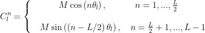
The first step in EIT is to apply currents on a finite set of electrodes around the boundary and measure the corresponding voltages obtained thereafter. Let L be the number of electrodes, then we can apply at most L-1 linearly independent current patterns (by current pattern we designate a vector of lenght L that describes the values of current applied in the electrodes). We designate by Cn the n-th current pattern. There are a few choices that can be considered for current patterns, but for now we fix our focus in two. For n=1,..., L-1 we have:
- Adjacent current patterns:
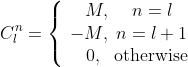
- Trignometric current patterns:
The corresponding voltages are denoted by Vn and each of them is a vector of dimension L (corresponding to the set of electrodes). One of the required assumptions is that for each current pattern the sum of the measured voltages equals zero. We assume that an EIT device provides the data in this manner.
For our algorithm we create a mapping from this data: Dirichlet-to-Neumman map, which establishes a relation between the Dirichlet boundary conditions (voltages) and the Neumann boundary conditions (currents) in conductivity model.
How to obtain the Dirichlet-to-Neumann map (DtoN map)?
-
Normalize the measurements:
cn= Cn/||Cn||2 and vn= Vn/||Cn||2
-
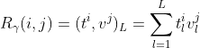
Define the Neumann-to-Dirichlet map (inverse of DtoN map), which is a L-1 x L-1 matrix:
- Compute the matrix approximation of Dirichlet-to-Neumann map for electrodes of Area A and a body of radius r:
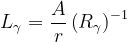
This mapping is the matrix approximation of the continuum operator for a body with conductivity γ.
Furthermore, the Dbar algorthm requires either the DtoN map of a body with the same geometry but with conductivity 1 or a reference DtoN map that corresponds to the same body with a different physiology (e.g. expiration and inspiration). This last case is designated by tdEIT and is very useful when monitoring health conditions that change with time like air ventilation in the lungs. With this in mind, the read_data class was constructed to compute one DtoN map from one set of current patterns and corresponding measured voltages.
Scattering Transform
The second step of the algorithm is to compute the scattering transform. This transform is of non-physical nature, i.e. has no physical explanation, but is tightly connect with the the conductivity and can be determined by the Dirichlet-to-Neumann map. It is given in the new spectral parameter k in the following manner:

Now due to the ill-posedness of the inverse problem, the noise in the measurements highly affects the values of t for large |k|. The regularization strategy proven by Siltanen shows that we only need to compute the following approximation for the scattering transform:
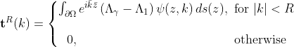
The beauty of this regularization strategy lies in a finite discretization of k inside a disk of radius R being required. The choice of R dependends in an estimate of the noise present in the measurements.
To completely understand the computation of the scattering transform we need to obtain ψ at the boundary. Nachman's was able to prove that the values of ψ at the boundary can be determined by the solution of a boundary integral equation for k ∈ ℂ \ {0}:

However, this equation takes a lot of time to solve, thus for speedup purposes we choose an approximate solution. We can have two approaches:
- Solve the boundary integral equation with S0 substituting Sk and with the following definition:

This approach is present in [2].
- Take ψ≃ e ikz, since this is the leading behavior and do not solve any integral equation. This is the fastest way, but its triviality leads to more errors.
Now the last step is to solve the Dbar equation, which gives the name to the algorithm.
D-bar equation
Now, having computed the scattering transform or an approximation of it, we are able to solve the following PDE in the k variable:

Afterwards, we can determine the conductivity by:
By substituting the scattering transform by its approximations and solving the equation with respect to it we obtain respective approximations to the conductivity.
5. Numerical Implementation
Above, we present an immediate numerical implementation of the Dirichlet-to-Neumann map that trivially translates to code and a theoretical implementation of the regularization strategy for the D-bar and corresponding determination of the conductivity. Accordingly, we present the numerical implementation for both versions of the scattering transform and the solution to the Dbar equation.
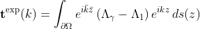
t-exp Scattering transform:
The t-exp scattering transform corresponds to take the exponential approximation of ψ, which has the following form:
Let us consider that we have equally distributed electrodes around the boundary. By our assumption of Ω being a disc we define, without loss of generality, the positions of the electrodes to be 

From this, we can take an approximation of the exponentials in these set points as an expansion in the orthonormal basis of current pattern (L-1 degrees of freedom):
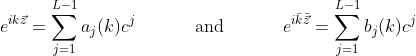
By immediate substitution and approximation of the integral at the electrode points this leads too:

t-B Scattering Transform:
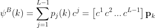
Here the first step is to solve the boundary integral equation with S0. For such we consider an initial vector approximation ψB of the solution of the (continuous) boundary integral equation and take the expansion in terms of the orthonormal current patterns:
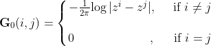
Further, we also take a LxL matrix approximation of G0 that defines the S0 operator as:
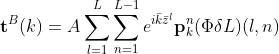
Through this matrix approximation, we can translate the boundary integral equation into a linear system of equations. Defining Φ to be the current pattern matrix (L x L-1) leads us too:

To compute the scattering transform we need to solve the last system of equations for each k in a disk of radius R. Afterwards, we compute it by:
A more in depth look at the details can be found in [1] with respect to the solution of the boundary integral equation with Sk.
D-bar Equation:
Now we have to solve the D-bar equation in the k-variable. This is the essence of this new spectral parameter, it allows for the reconstruction of the conductivity without iterative solutions of an FEM model of conductivity. Although, we do not solve the PDE directly... we pass it to an integral equation and use Fourier Transform after discretization to solve the linear system of equations.
Integral Equation:
Solve for each z∈Ω:
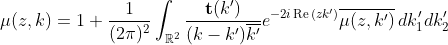
Recall that, the regularization procedure establishes that for |k|>R the scattering transform is 0, in both cases. Hence, the integral can be taken in the disk of radius R. To practically solve this equation we need to deal with the singularity properly. A fast approach to solve the equation is to transform it into a periodic setting (initial idea was by Vainikko, [3], and adapted to the Dbar equation in [4]). Let 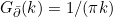

The periodization is done by tiling the k-plane with a square Q=[-2R-3ε, 2R + 3ε]2 for some ε>0, in this manner, Q containes the disk of radius 2R. Now, we take a smooth cut-off function η which fulfils η(k)=1 for |k|<2R+ε and η(k)=0 for |k|>2R+2ε. With this we define the periodic approximate green function 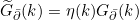
In this framework we have the periodic version of the integral D-bar equation given by:
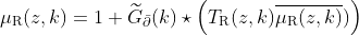
where ⋆ denotes periodic convolution and TR is the defined as T for |k|<R and 0 otherwise. The interesting part is that the solution of this equation and of the full equation coincide in |k|<R, which is what we desire.
By discretizing the k-plane into an equally spaced grid with step h, the periodic convolution can be computed efficiently by Fast Fourier transforms and we obtain the following system of equations:

where the boldface notation represents the matrices formed by evaluation of the functions in the k-grid and ⋅ represents matrix multiplication. This equation can be written in a simpler form, which will be helpful to describe our code below:

Since μR is inside the Fourier transform, we can not describe this system through the simple form Ax=b. Hence, the system of equations lends itself well to a solution by a matrix-free iterative solver like the GMRES.
Due to conjugation on μR the equation is ℝ-linear and separation of the real and imaginary parts, which is done by justposition of the real and imaginary parts into a vector. Further details, can be seen in [1].
This is what we need for implementation and it provides a framework for the code we present in this package. A description of each class and function and its role is presented next.
6. Documentation:
Here, we provide an overview of each class and examples of usage. Our package possesses three classes:
sim, read_data, k_grid, scattering, dBar.
The first three classes are independent and concern the input information and framework. The fourth connects the gather data into a single operator, which is transmitted to the dBar class. This class is dependent of both the scattering and k_grid and performs the solver.
sim class
class sim(anomaly, L)
This class is a simulator of voltages obtained through the FEM-solution of the Direct problem. We can create the conductivity of a body in a disk and then solve the direct problem for this conductivity by applying pair-wise adjacent current patterns (as described above). Thereafter, we can determine the voltage at the electrode positions and hence create the necessary data to apply an inversion procedure.
This class is based solely on pyEIT.
Parameters:
-
anomaly: list
By assumption we have that the background conductivity is equal to 1. Then we can create disk anomalies by selecting the center, radius and the conductivity of the region.
-
L: int
Number of electrodes.
Attributes:
-
Current: (L-1, L)
Matrix with the currents patterns applied to the body.
-
Voltage: (L-1, L)
Matrix with the "measured" voltages obtained to sucessive FEM-solutions of the direct problem.
Methods:
-
simulate():
This function uses each of the adjacent pair current patterns, solves the direct problem by FEM, and determines the voltages at the electrodes.
read_data class
class read_data(Object, r, AE, L)
Defines the Dirichlet-to-Neumann matrix approximation from the experimental data: electrical measurements, radius of the body, area of electrode and number of electrodes. The current version only holds for circular domains and for objects which have conductivity equal to 1 near the boundary.
Parameters:
-
Current: (L-1, L) 2darray
Matrix of current patterns. Each line is a current pattern.
-
Voltage: (L-1, L) 2darray
Matrix of voltage measurements. Each line corresponds to the current pattern on the same line of the current matrix.
-
r: float
Radius of the body;
-
AE: float
Area of one electrode;
-
L: int
Number of electrodes;
Attributes:
-
Current: (L, L-1) 2darray
Matrix of the normalized current patterns, each column represents one normalized current pattern;
-
Voltage: (L, L-1) 2darray
Matrix of the normalized voltages, where the i-th column represents the voltages measured for the i-th current pattern;
-
DNmap: (L-1, L-1) 2darray
Matrix approximation of Dirichlet-to-Neumann map for the measured data.
Methods:
-
load():
This function starts by performing the normalization of the current and voltage measurements and thereafter computes the Dirichlet-to-Neumann as described above. It is called directly from the constructor and the user does need to use it directly.
Examples:
k_grid class
class k_grid(R, m)
Definition of the grid discretization of the k-plane with respect to the parameters R and m. As required by the periodic discrete convolution, the grid is defined in [-2.3R, 2.3R]^2 with step size h=2(2.3R)/2m.
Parameters:
-
R: float
Defines the size of the k grid
-
m: int
Defines the step size.
Attributes:
-
R: float
As the parameter.
-
m: int
As the parameter.
-
s: float
It is defined as 2.3R, to simplify definitions further ahead.
-
h: float
Step size of the k grid.
-
N: int
It is defined as 2m. Therefore, it is the number of elements on each line of the grid.
-
k: (N, N) complex 2darray
Complex values of the k_grid. Essential for complex-valued computations. This grid contains the value 0.
-
pos_x, pos_y: array_like
Arrays that store the indexes of the elements of k which are inside the disk of radius R.
-
index: int
Represents the position of zero.
-
FG: (N, N) complex 1darray
The fundamental solution
of the D-bar operator, with the same structure of k.
Methods:
-
generate():
Defines the complex k-grid k and determines the positions inside the disk of radius R.
-
Green_FS():
Defines the FFT of fundamental solution FG. Recall that we perform a periodization of the convolution equation and therefore we need to establish a smooth decay to 0 close to the square limits of the grid.
scattering class
class scattering(scat_type, k_grid, Now, Ref):
Parameters:
-
scat_type: string
Allows to choose between the approximations of the scattering transform. Choices: "partial", "exp"!.
-
k_grid: Object
An object of k_grid type.
-
Now, Ref: Objects
Objects of read_data type (we require the DN map for our body of choice and an homogeneous/reference body).
Attributes:
-
tK: (k_grid.N, k_grid.N) complex 2darray
Matrix containing the values of an intermediare operator containing information about the DN map of our body of choice. Essential for the Dbar method.
Methods:
-
load_scattering(scat_type, k_grid, Now, Ref):
Given the choice of approximation for the scattering transform this function selects between two functions: one compute the exponential aproximation, another computes the partial approximation;
-
exp_scattering(Now, Ref, k_grid):
Computes the exponential approximation of the scattering transform.
-
partial_scattering(Now, Ref, k_grid):
Computes the partial approximation of the scattering transform.
dBar class
class dBar(R_z, m_z)
Parameters:
-
R_z: float
Defines the size of the z-grid.
-
m_z: int
Defines the step size of the z-grid.
Attributes:
-
Z: (2m_z, 2m_z) complex 2darray
Planar region of the body.
-
sigma: (2m_z, 2m_z) complex 2darray
Conductivity values at the points of the Z-plane grid.
Methods:
-
load_mesh(R, m):
Defines the complex z-grid Z.
-
dBar(mu, k_grid, tK, zz):
Defines the operator [I + P] for a zz element of the z-grid, which is the left-hand side of the Dbar system. It takes as input the vector μ which is a 1darray that contains the real part concatenated with the imaginary part. We assume μ is 0 outside the disk of radius R, for speed-up purposes, however this is not a constraint since the scattering transform would cut-off this terms when defining the operator.
-
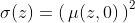
solve(k_grid, tK):
Solve for each z on the z-grid the Dbar system with GMRES. We use the dBar function to define the [I+P] operator for each z and use the initial approximation of mu being close to 1 to start off. After solving the system, we store the value of the conductivity through γ(z)=(μ(z,0))^2.
-
plot():
Plot the obtained conductivity on the respective Z grid.
6. Bibliography:
[1] Mueller, J. L., & Siltanen, S. (2020). The d-bar method for electrical impedance tomography—demystified. Inverse problems, 36(9), 093001.
[2] El Arwadi, T., & Sayah, T. (2021). A new regularization of the D-bar method with complex conductivity. Complex Variables and Elliptic Equations, 66(5), 826-842.
[3] Vainikko, G. (2000). Fast solvers of the Lippmann-Schwinger equation. In Direct and inverse problems of mathematical physics (pp. 423-440). Springer, Boston, MA.
[4] Knudsen, K., Mueller, J., & Siltanen, S. (2004). Numerical solution method for the dbar-equation in the plane. Journal of Computational Physics, 198(2), 500-517.
Release history Release notifications | RSS feed


Download files
Download the file for your platform. If you're not sure which to choose, learn more about installing packages.
Source Distribution
Built Distribution
Filter files by name, interpreter, ABI, and platform.
If you're not sure about the file name format, learn more about wheel file names.
Copy a direct link to the current filters
File details
Details for the file py_dbar-1.0.0.tar.gz.
File metadata
- Download URL: py_dbar-1.0.0.tar.gz
- Upload date:
- Size: 22.8 kB
- Tags: Source
- Uploaded using Trusted Publishing? No
- Uploaded via: twine/3.4.2 importlib_metadata/4.6.1 pkginfo/1.5.0.1 requests/2.24.0 requests-toolbelt/0.9.1 tqdm/4.47.0 CPython/3.8.3
File hashes
| Algorithm | Hash digest | |
|---|---|---|
| SHA256 |
2f5b4dff675bff487c359b4402d8c47b73c4c4e889fa3403c3df8b380e7b3b7d
|
|
| MD5 |
0c6a32d367b170da62a4663c81ffabc9
|
|
| BLAKE2b-256 |
a2a5fb387ed1f52e65b117c7ba1e0d92ce2fd9328e33071ff89ae7d4f31d7908
|
File details
Details for the file py_dbar-1.0.0-py3-none-any.whl.
File metadata
- Download URL: py_dbar-1.0.0-py3-none-any.whl
- Upload date:
- Size: 16.0 kB
- Tags: Python 3
- Uploaded using Trusted Publishing? No
- Uploaded via: twine/3.4.2 importlib_metadata/4.6.1 pkginfo/1.5.0.1 requests/2.24.0 requests-toolbelt/0.9.1 tqdm/4.47.0 CPython/3.8.3
File hashes
| Algorithm | Hash digest | |
|---|---|---|
| SHA256 |
f85afc226103232a1148725e8aef3e96c0c341710fcfce4c6d6dab8454590073
|
|
| MD5 |
3c356225c99f8885a3c6debfbde84b99
|
|
| BLAKE2b-256 |
af01050c63fd0f740d10f13ca4c4eee6ba99ea7a8b184671c64b248f07aa874f
|


