python utilities for working with the VBRc

Project description


pyVBRc
pyVBRc is a python package for working with output from the Very Broadband Rheology Calculator. pyVBRc is currently (very) experimental and is likely to change drastically between early versions, but feel free to use it.
Installation
To install the latest release:
pip install pyVBRc
To install the latest development version, see the section on Contributing.
Usage
As of now, the primary uses of the pyVBRc are to:
- load a VBR structure
- interpolate between calculated values in the VBR structure
Loading a VBR structure
The primary gateway into working with VBRc data is the VBRstruct object.
Note that the following examples rely on a tiny VBR output file, VBRc_sample_LUT.mat, included in pyVBRc to allow
simple testing of functionality. For any real application, you should generate your own VBR structure (in MATLAB or Octave).
The most basic usage of the VBRCstruct object is to load a .mat file containing a VBR structure that you have saved:
from pyVBRc.vbrc_structure import VBRCstruct
from pyVBRc.sample_data import get_sample_filename
file = get_sample_filename("VBRc_sample_LUT.mat")
vbr = VBRCstruct(file)
The vbr object will mirror the standard VBR structure (see here)
with the exception that the in and out structures of the matlab VBR structure are replaced with input and output
in the python class.
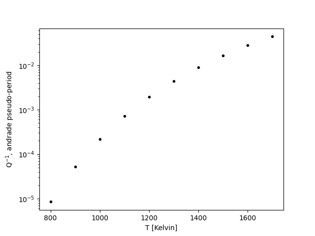
Once loaded, you can access the data just as in matlab. This .mat file contains a VBR structure that was run with
varying temperature (T_K), melt fraction (phi) and grain size(dg_um) at two frequencies. The following example
plots the temperature dependence of attenuation for the Andrade pseuodo-period scaling at a fixed grain size,
melt fraction and frequency:
import matplotlib.pyplot as plt
T_K = vbr.input.SV.T_K[:, 0, 0]
Qinv = vbr.output.anelastic.andrade_psp.Qinv[:, 0, 0, 0]

plt.semilogy(T_K, Qinv, '.k')
plt.xlabel("T [Kelvin]")
plt.ylabel("Q^{-1}, andrade pseudo-period")
plt.show()
Interpolating
In some situations, it may be useful to interpolate VBRc results at arbitrary points between calculated points. The sample file,"VBRc_sample_LUT.mat" was calculated for a very coarse grid of temperature (T_K), melt fraction (phi) and grain size(dg_um) at two frequencies to serve as a simple look-up table (LUT). You can provide these variable names to the lut_dimensions keyword argument when initializing the VBRCstruct:
from pyVBRc.vbrc_structure import VBRCstruct
from pyVBRc.sample_data import get_sample_filename

file = get_sample_filename("VBRc_sample_LUT.mat")
vbr = VBRCstruct(file, lut_dimensions=["T_K", "phi", "dg_um"])
Now, you can build a grid interpolator for a single method-array and a single frequency index with the interpolator method. This method also accepts the log_vars keyword argument that you can use to specify LUT fields that you want to interpolate in log-space:
import numpy as np
interp = vbr.interpolator(
    ("anelastic", "andrade_psp", "V"), 0, log_vars=["phi", "dg_um"]
)

# evaluate at one arbitrary point
# (T in K, log(phi), log(dg in micrometer))
target = (1333 + 273.0, np.log10(0.0012), np.log10(1131))

Vs_interp = interp(target)
print(Vs_interp)
Note that the array to interpolate is specified as a tuple of output fieldnames: ("anelastic", "andrade_psp", "V") corresponds to accessing VBR.output.anelastic.andrade_psp.V. To interpolate at more than one point, you can provide an array of points:
import matplotlib.pyplot as plt
# resample at a higher resolution
T = vbr.input.SV.T_K[:, 0, 0]
nT = len(T)
T_targets = np.linspace(T.min(), T.max(), nT * 2)
phival = vbr.input.SV.phi.min()
dgval = vbr.input.SV.dg_um.min()
phi_targets = np.full(T_targets.shape, np.log10(phival))
dg_targets = np.full(T_targets.shape, np.log10(dgval))
targets = np.column_stack((T_targets, phi_targets, dg_targets))
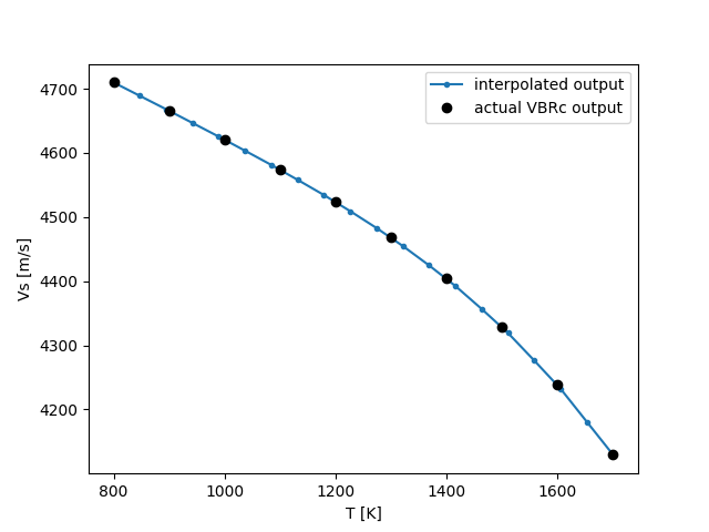
Vs_interp = interp(targets)
# compare to actual Vs along curve
actual_Vs = vbr.output.anelastic.andrade_psp.V[:, 0, 0, 0]
plt.plot(T_targets, Vs_interp, label="interpolated output", marker=".")
plt.plot(T, actual_Vs, ".k", label="actual VBRc output", markersize=12)
plt.legend()
plt.xlabel("T [K]")
plt.ylabel("Vs [m/s]")
plt.show()
which yields
NOTE that the validity of any interpolation will depend on the underlying VBR structure that you have built.
Isotropic Mixtures and Anistropy
The pyVBRc includes some limited functionality for calculating properties of Isotropic mixture as well as
anistropic properties. See the Examples for a description.
Examples
The examples directory contains a number of jupyter notebooks that demonstrate usage.
Getting help
If you find a bug, please open an issue.
If you have questions, feel free to ask in the VBRc slack channel (see here for how to join.)
Contributing
Contributions fall a fork-pull request open source work flow:
- Fork this repository
- Clone your fork and build a development installation (see below)
- Create a new branch (
git checkout -b your_new_branch_name) - Commit changes on your branch
- Push your branch to your fork
- Submit pull request (PR) to the main
pyVBRcrepository
After PR submission, a number of automated tests will run and your changes will be reviewed. Often this may involve some iteration, but we'll help you out if you're new to git!
Development installation
After cloning your fork, you can install pyVBRc with
pip install -e .[dev]
and then install all the development requirements with
pip install -r requirements_dev.txt
running the test suite
After completing your development installation, you can run the test suite with
pytest -v
To also generate a code coverage report
pytest -v --cov=./ --cov-report=html:coverage/
After tests run, you can then open the coverage/index.html file in your
preferred browser and check out where test coverage is poor.
Pull requests are required to maintain the code coverage of the code base, so you'll have to write new tests to cover any new code. Bug fixes may not require new tests if coverage is unchanged.
code style
style checks
Code style is enforced with pre-commit. When you submit a pull request, the
pre-commit.ci bot will test whether your code passes the style requirements. If
that test fails, you can have pre-commit.ci autofix your pull request by adding
a comment to the pull request that reads
pre-commit.ci autofix
and the bot will try to fix the style failures. After it runs, if you still have work to do on the PR, you'll want to run
git pull
locally so that you can pull in the bot's changes to your branch.
using pre-commit during development
If you'd like to ensure that your code passes all style requirements while you're developing, you can use pre-commit throughout development. After building your development installation, you can initialize pre-commit within your repository with
pre-commit install
and your code changes will be checked every time you commit.


Download files
Download the file for your platform. If you're not sure which to choose, learn more about installing packages.
Source Distribution
Built Distribution
Filter files by name, interpreter, ABI, and platform.
If you're not sure about the file name format, learn more about wheel file names.
Copy a direct link to the current filters
File details
Details for the file pyVBRc-0.3.2.tar.gz.
File metadata
- Download URL: pyVBRc-0.3.2.tar.gz
- Upload date:
- Size: 779.0 kB
- Tags: Source
- Uploaded using Trusted Publishing? No
- Uploaded via: twine/4.0.2 CPython/3.11.7
File hashes
| Algorithm | Hash digest | |
|---|---|---|
| SHA256 |
9d620c50bc41338e969f249dfc027e088b722c00f8e4f5bbb0678752822bd16e
|
|
| MD5 |
412abfbc5a4e50243fa2486be63640e7
|
|
| BLAKE2b-256 |
ee51ab612140c2b0861fa7d6852b06d68f8897ff3a2b68b336b061cca3a6d6cc
|
File details
Details for the file pyVBRc-0.3.2-py3-none-any.whl.
File metadata
- Download URL: pyVBRc-0.3.2-py3-none-any.whl
- Upload date:
- Size: 775.4 kB
- Tags: Python 3
- Uploaded using Trusted Publishing? No
- Uploaded via: twine/4.0.2 CPython/3.11.7
File hashes
| Algorithm | Hash digest | |
|---|---|---|
| SHA256 |
caae48e01df52957c494bb3fbb2f81222d645cc70519e2e5533254b9870bb19d
|
|
| MD5 |
111a4482fafd12412c048ca9d92933b2
|
|
| BLAKE2b-256 |
79f3e7d0b84bc2f97ddade4e09682b55bae8d6b777236c6f862c3cff0c6c2354
|


