Simulation package for the propagation of optical pulses in nonlinear media

Project description
pychi
A Python package for simulating the propagation of optical pulses in nonlinear materials.
Capabilities
pychi is aimed at simulating the propagation of short pulses in nonlinear media and capturing as much physics as possible. It is based on a unidirectional propagation model, which stays valid even for sub-cycle optical pulses. In particular, this propagation model accounts for
- Full frequency dependence of the effective refractive index
- Quadratic nonlinear interactions (sum- and difference-frequency generation)
- Cubic nonlinear interactions (triple sum-frequency generation, self-phase modulation, conjugated Kerr term)
- Raman scattering
- Self-steepening
- Frequency-dependence of the nonlinear coefficients and effective area
- z-dependence of the effective refractive index, nonlinear coefficients and effective area (permitting poling to be simulated)
The package is built to be as user-friendly as possible, providing a relatively high-level interface for the user while still allowing for physically intricate simulation cases. It leverages a custom-made order 5 solver, although more classical solvers (such as the RK4IP) have also been implemented for completeness and versatility.
Installation
First, make sure pip is up-to-date using
pip install --upgrade pip
On Windows, install the package using
pip install pychi
On Mac, one might have to first run
conda install -c conda-forge pyfftw
due to some OS specificities in pyFFTW installation.
Then, one should be able to install pychi normally using
pip install pychi
Documentation
The documentation is available and best viewed under https://pychi.readthedocs.io/en/latest/ This documentation has been automatically generated using SPHINX, and is still a work in progress. Do not hesitate to contact us for any needed clarifications and examples.
Implementation
pychi has been developped at DESY by the Ultrafast Microphotonics group. Details about the implementation have been published at https://doi.org/10.1063/5.0135252 - if you use pychi for scientific publications, please cite this paper.
Theory
The full theoretical derivation leading to the master equation used in pychi is described in Appendix C of the following thesis: https://ediss.sub.uni-hamburg.de/handle/ediss/10785.
Example
Here is a typical example of the use of pychi to simulate the propagation of a short optical pulse in a nonlinear waveguide exhibiting both cubic and quadratic nonlinearities.
# -*- coding: utf-8 -*-
"""
Created on Mon Feb 28 15:31:47 2022
The waveguide/fiber parameters are first provided, and a Waveguide instance
is created. Then, the pulse parameters are used to create a Light object.
A physical model is then chosen, taking into account different nonlinear
interactions based on the user choice. Finally, a solver is instantiated
and computes the propagation of the pulse in the waveguide with the chosen
nonlinear interactions.
@author: voumardt
"""
import matplotlib.pyplot as plt
import numpy as np
from scipy.constants import c

import pychi


"""
User parameters
"""
### Simulation
t_pts = 2**15

### Light
pulse_duration = 100e-15
pulse_wavelength = 1.56e-06
pulse_energy = 1e-9

### Waveguide
wg_length = 0.001
wg_chi_2 = 1.1e-12
wg_chi_3 = 3.4e-21
wg_a_eff = 1e-12
wg_freq, wg_n_eff = np.load('effective_index.npy')
# wg_n_eff is the effective dispersion of the waveguide considered, sampled on the grid wg_freq


"""
Nonlinear propagation
"""
### Prepare waveguide
waveguide = pychi.materials.Waveguide(wg_freq, wg_n_eff, wg_chi_2, wg_chi_3,
                                wg_a_eff, wg_length, t_pts=t_pts)
# Additional options:
# wg_n_eff can be a 2 dimensional array, with first dimension the wavelength dependence
# and second dimension the z dependence.
#
# chi2 and chi3 can be callables, returning a z dependent value. Alternatively, they
# can be defined as one dimensional arrays describing their z dependence, or
# two dimensional arrays describing their z and frequency dependence. They
# can also be callables of (z, freq).
#
# One can use waveguide.set_gamma(gamma) or waveguide.set_n2(n2) to provide a
# nonlinear coefficient or nonlinear refractive index and overwrite chi3.
#
# Check documentation for more options and details.


### Prepare input pulse
pulse = pychi.light.Sech(waveguide, pulse_duration, pulse_energy, pulse_wavelength)
# Other available pulse shapes:
# pulse = pychi.light.Gaussian(waveguide, pulse_duration, pulse_energy, pulse_wavelength)
# pulse = pychi.light.Cw(waveguide, pulse_average_power, pulse_wavelength)
# pulse = pychi.light.Arbitrary(waveguide, pulse_frequency_axis, pulse_electric_field, pulse_energy)


### Prepare model
model = pychi.models.SpmChi2Chi3(waveguide, pulse)
# Other models available:
# model = pychi.models.Spm(waveguide, pulse)
# model = pychi.models.Chi2(waveguide, pulse)
# model = pychi.models.Chi3(waveguide, pulse)
# model = pychi.models.SpmChi2(waveguide, pulse)
# model = pychi.models.SpmChi3(waveguide, pulse)
# model = pychi.models.Chi2Chi3(waveguide, pulse)


### Prepare solver, solve
solver = pychi.solvers.Solver(model)
solver.solve()


"""
Plots
"""
pulse.plot_propagation()
# Results can also be accessed via pulse.z_save, pulse.freq, pulse.spectrum, pulse.waveform
# The refractive index and GVD can be seen with waveguide.plot_refractive_index()
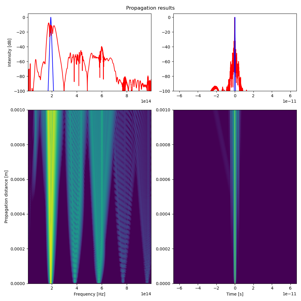
Typical propagation results using the above script would look as follows:
Check the examples folder for some specific cases and validation against experimental data.
Contacts
If you have any questions, remarks, contributions, do not hesitate to contact us at: pychi@desy.de or here on GitHub.
Project details
Release history Release notifications | RSS feed


Download files
Download the file for your platform. If you're not sure which to choose, learn more about installing packages.
Source Distribution
Built Distribution
Filter files by name, interpreter, ABI, and platform.
If you're not sure about the file name format, learn more about wheel file names.
Copy a direct link to the current filters
File details
Details for the file pychi-0.0.20.tar.gz.
File metadata
- Download URL: pychi-0.0.20.tar.gz
- Upload date:
- Size: 20.4 kB
- Tags: Source
- Uploaded using Trusted Publishing? No
- Uploaded via: twine/6.1.0 CPython/3.13.5
File hashes
| Algorithm | Hash digest | |
|---|---|---|
| SHA256 |
76342f0300f1d79d93f532029579d43ae255c4d7683609bfd69726a4df5e07e7
|
|
| MD5 |
43af54de65d5d05b74b618ad53d289ba
|
|
| BLAKE2b-256 |
578cb0f35110c3a07da45997683fd62f422d2e704df3c322fae075a3183316d6
|
File details
Details for the file pychi-0.0.20-py3-none-any.whl.
File metadata
- Download URL: pychi-0.0.20-py3-none-any.whl
- Upload date:
- Size: 20.2 kB
- Tags: Python 3
- Uploaded using Trusted Publishing? No
- Uploaded via: twine/6.1.0 CPython/3.13.5
File hashes
| Algorithm | Hash digest | |
|---|---|---|
| SHA256 |
d6c2f42f7234c1f3cf4fc9980e39f40e2c14b09fc027c920a33c8ebfc4358174
|
|
| MD5 |
74a972c275b402ee62dbad367715dab0
|
|
| BLAKE2b-256 |
539513d592100e8137a690b0a520363ed01737b80ba8ff6c192f95637b454c42
|


