




Overview
Pycop is the most complete tool for modeling multivariate dependence with Python. The package provides methods such as estimation, random sample generation, and graphical representation for commonly used copula functions. The package supports the use of mixture models defined as convex combinations of copulas. Other methods based on the empirical copula such as the non-parametric Tail Dependence Coefficient are given.
Some of the features covered:
- Elliptical copulas (Gaussian & Student) and common Archimedean Copulas functions
- Mixture model of multiple copula functions (up to 3 copula functions)
- Multivariate random sample generation
- Empirical copula method
- Parametric and Non-parametric Tail Dependence Coefficient (TDC)
Available copula function
| Copula | Bivariate Graph & Estimation |
Multivariate Simulation |
|---|---|---|
| Mixture | ✓ | ✓ |
| Gaussian | ✓ | ✓ |
| Student | ✓ | ✓ |
| Clayton | ✓ | ✓ |
| Rotated Clayton | ✓ | ✓ |
| Gumbel | ✓ | ✓ |
| Rotated Gumbel | ✓ | ✓ |
| Frank | ✓ | ✓ |
| Joe | ✓ | ✓ |
| Rotated Joe | ✓ | ✓ |
| Galambos | ✓ | ✗ |
| Rotated Galambos | ✓ | ✗ |
| BB1 | ✓ | ✗ |
| BB2 | ✓ | ✗ |
| FGM | ✓ | ✗ |
| Plackett | ✓ | ✗ |
| AMH | ✗ | ✓ |
Usage
Install pycop using pip
pip install pycop
Examples

Table of Contents
Graphical Representation
We first create a copula object by specifying the copula familly
from pycop import archimedean
cop = archimedean(family="clayton")
Plot the cdf and pdf of the copula.
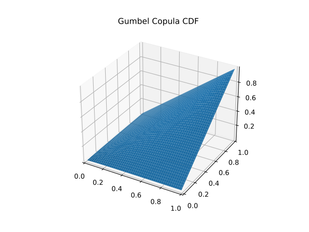
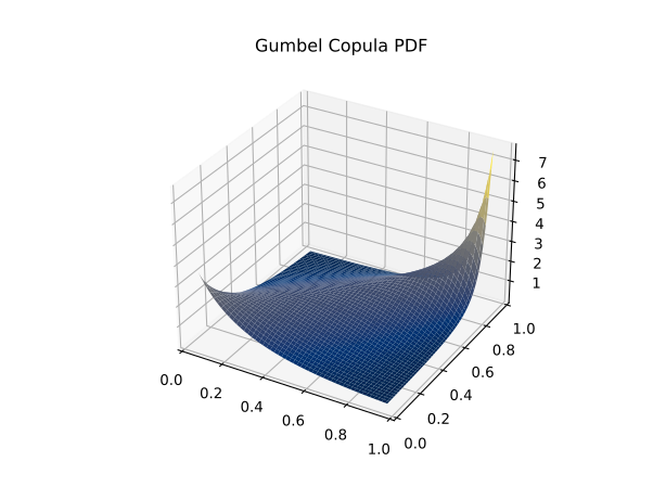
3d plot
cop = archimedean(family="gumbel")

cop.plot_cdf([2], plot_type="3d", Nsplit=100 )
cop.plot_pdf([2], plot_type="3d", Nsplit=100, cmap="cividis" )
Contour plot
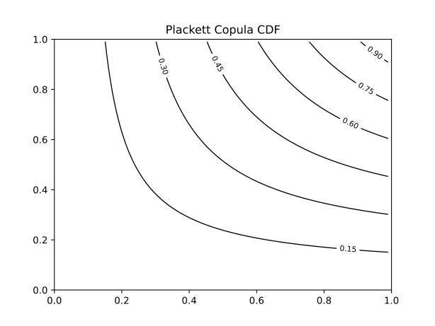
plot the contour
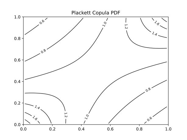
cop = archimedean(family="plackett")

cop.plot_cdf([2], plot_type="contour", Nsplit=100 )
cop.plot_pdf([2], plot_type="contour", Nsplit=100, )
It is also possible to add specific marginals
cop = archimedean.archimedean(family="clayton")

from scipy.stats import norm


marginals = [
    {
        "distribution": norm, "loc" : 0, "scale" : 0.8,
    },
    {
        "distribution": norm, "loc" : 0, "scale": 0.6,
    }]

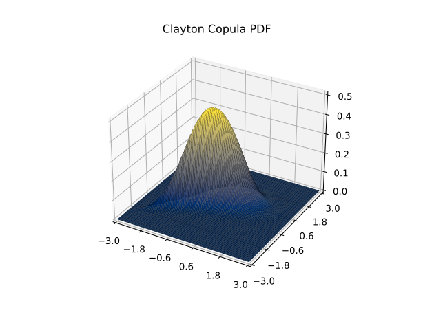
cop.plot_mpdf([2], marginals, plot_type="3d",Nsplit=100,
            rstride=1, cstride=1,
            antialiased=True,
            cmap="cividis",
            edgecolor='black',
            linewidth=0.1,
            zorder=1,
            alpha=1)

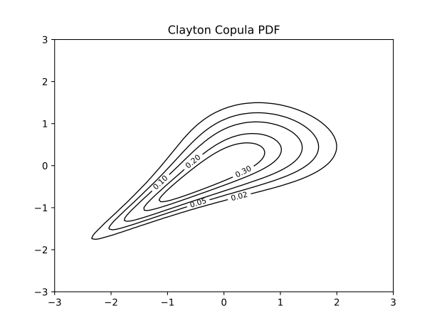
lvls = [0.02, 0.05, 0.1, 0.2, 0.3]

cop.plot_mpdf([2], marginals, plot_type="contour", Nsplit=100,  levels=lvls)
Mixture plot
mixture of 2 copulas
from pycop import mixture

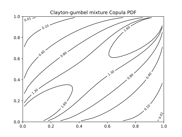
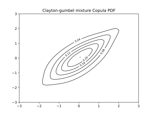
cop = mixture(["clayton", "gumbel"])
cop.plot_pdf([0.2, 2, 2],  plot_type="contour", Nsplit=40,  levels=[0.1,0.4,0.8,1.3,1.6] )
# plot with defined marginals
cop.plot_mpdf([0.2, 2, 2], marginals, plot_type="contour", Nsplit=50)
cop = mixture(["clayton", "gaussian", "gumbel"])
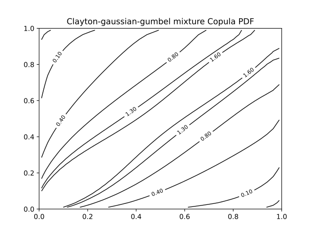
cop.plot_pdf([1/3, 1/3, 1/3, 2, 0.5, 4],  plot_type="contour", Nsplit=40,  levels=[0.1,0.4,0.8,1.3,1.6] )
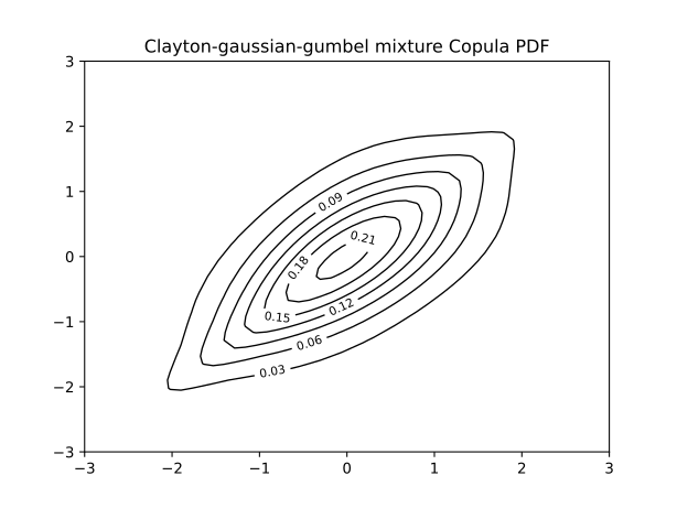
cop.plot_mpdf([1/3, 1/3, 1/3, 2, 0.5, 2], marginals, plot_type="contour", Nsplit=50)
Simulation
Gaussian
from scipy.stats import norm
from pycop import simulation

n = 2 # dimension
m = 1000 # sample size

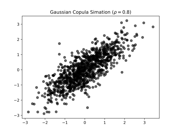
corrMatrix = np.array([[1, 0.8], [0.8, 1]])
u1, u2 = simulation.simu_gaussian(n, m, corrMatrix)
Adding gaussian marginals, (using distribution.ppf from scipy.statsto transform uniform margin to the desired distribution)
u1 = norm.ppf(u1)
u2 = norm.ppf(u2)
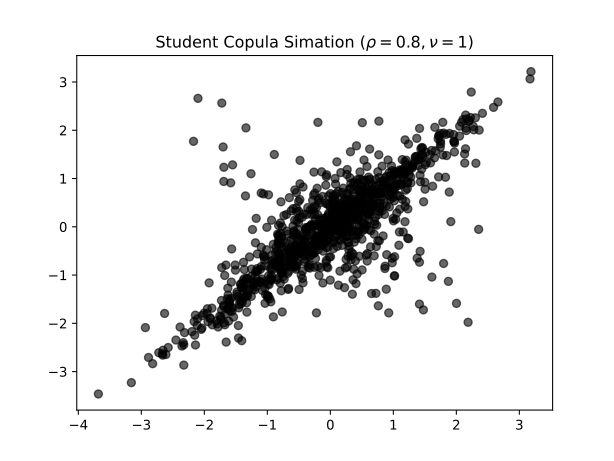
Student
u1, u2 = simulation.simu_tstudent(n, m, corrMatrix, nu=1)
Archimedean
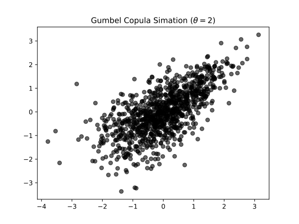
List of archimedean cop available
u1, u2 = simulation.simu_archimedean("gumbel", n, m, theta=2)
u1, u2 = 1 - u1, 1 - u2
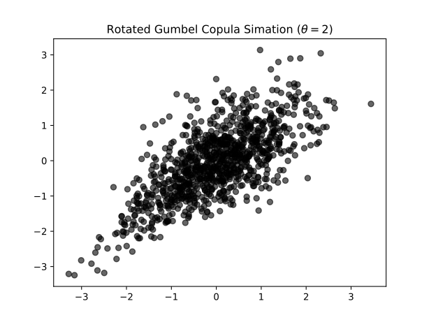
Rotated
u1, u2 = 1 - u1, 1 - u2
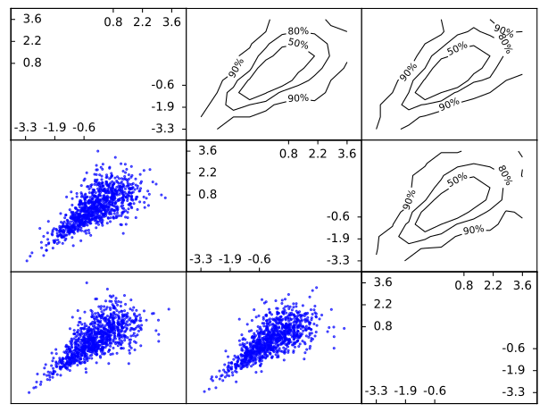
High dimension
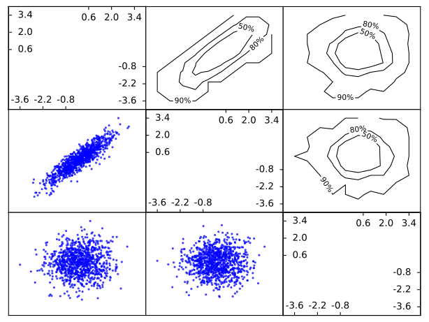
n = 3       # Dimension
m = 1000    # Sample size

corrMatrix = np.array([[1, 0.9, 0], [0.9, 1, 0], [0, 0, 1]])
u = simulation.simu_gaussian(n, m, corrMatrix)
u = norm.ppf(u)
u = simulation.simu_archimedean("clayton", n, m, theta=2)
u = norm.ppf(u)
Mixture simulation
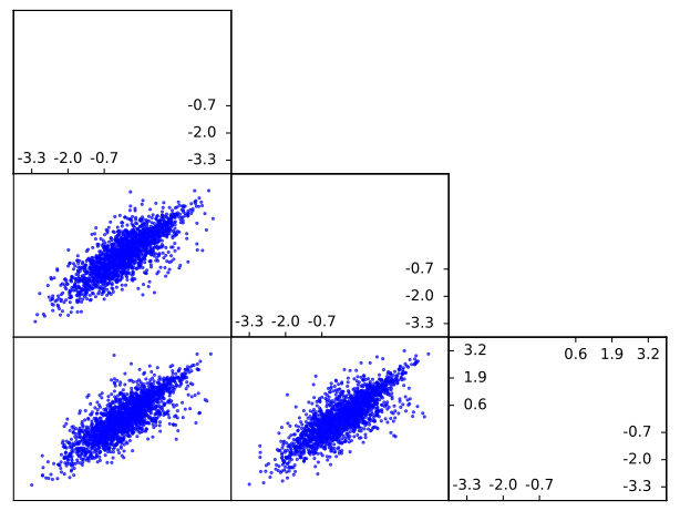
Simulation from a mixture of 2 copulas
n = 3
m = 2000

combination = [
    {"type": "clayton", "weight": 1/3, "theta": 2},
    {"type": "gumbel", "weight": 1/3, "theta": 3}
]

u = simulation.simu_mixture(n, m, combination)
u = norm.ppf(u)
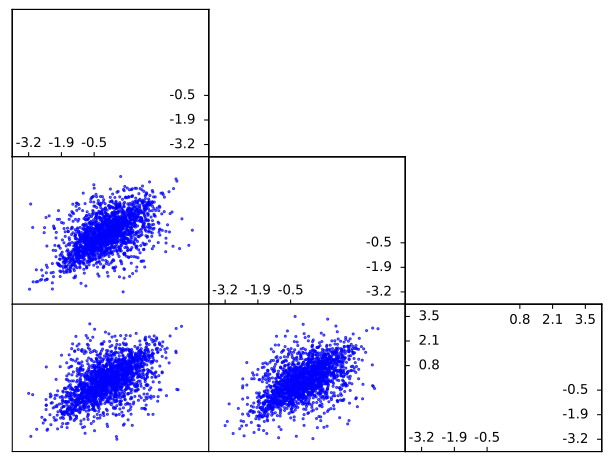
Simulation from a mixture of 3 copulas
corrMatrix = np.array([[1, 0.8, 0], [0.8, 1, 0], [0, 0, 1]])


combination = [
    {"type": "clayton", "weight": 1/3, "theta": 2},
    {"type": "student", "weight": 1/3, "corrMatrix": corrMatrix, "nu":2},
    {"type": "gumbel", "weight": 1/3, "theta":3}
]

u = simulation.simu_mixture(n, m, combination)
u = norm.ppf(u)
Estimation
Estimation available : CMLE
Canonical Maximum Likelihood Estimation (CMLE)
Import a sample with pandas
import pandas as pd
import numpy as np

df = pd.read_csv("data/msci.csv")
df.index = pd.to_datetime(df["Date"], format="%m/%d/%Y")
df = df.drop(["Date"], axis=1)

for col in df.columns.values:
    df[col] = np.log(df[col]) - np.log(df[col].shift(1))

df = df.dropna()
from pycop import estimation, archimedean

cop = archimedean("clayton")
data = df[["US","UK"]].T.values
param, cmle = estimation.fit_cmle(cop, data)
clayton estim: 0.8025977727691012
Tail Dependence coefficient
Theoretical TDC
from pycop import archimedean

cop = archimedean("clayton")

cop.LTDC(theta=0.5)
cop.UTDC(theta=0.5)
For a mixture copula, the copula with lower tail dependence comes first, and the one with upper tail dependence is last.
from pycop import mixture

cop = mixture(["clayton", "gaussian", "gumbel"])

LTDC = cop.LTDC(weight = 0.2, theta = 0.5)
UTDC = cop.UTDC(weight = 0.2, theta = 1.5)
Non-parametric TDC
Create an empirical copula object
from pycop import empirical

cop = empirical(df[["US","UK"]].T.values)
Compute the non-parametric Upper TDC (UTDC) or the Lower TDC (LTDC) for a given threshold:
cop.LTDC(0.01) # i/n = 1%
cop.UTDC(0.99) # i/n = 99%
Optimal Empirical TDC
Returns the optimal non-parametric TDC based on the heuristic plateau-finding algorithm from Frahm et al (2005) "Estimating the tail-dependence coefficient: properties and pitfalls"
cop.optimal_tdc("upper")
cop.optimal_tdc("lower")
1 maintainer

Release files for pycop 0.0.13
For a detailed explanation of source distributions (sdists) and built distributions (wheels), please see the package formats documentation.
Source distribution (sdist)
| File | Size | Uploaded | |
|---|---|---|---|
| pycop-0.0.13.tar.gz | 20.4 kB | Details |
Built distribution (wheel)
| File | Interpreter | ABI | Platform | Reset |
|---|---|---|---|---|
| pycop-0.0.13-py3-none-any.whl | Python 3 | none | any | Details |
Total release size: 42.4 kB
Release files / pycop-0.0.13.tar.gz
| Download URL | pycop-0.0.13.tar.gz |
|---|---|
| Size | 20.4 kB |
| Tags | Source |
|
SHA-256 checksum How to use checksums |
c52e89dc3c003f1f42b5e7820a4a0728cc130b3ae57b46eeeb871f20398847e1
|
|
BLAKE2b-256 checksum How to use checksums |
69eeb7ea9043a60f5f91ce254313d587aa9d6a17f3bd0e93be9fcb74f9d7102c
|
| Upload date | |
|
Uploaded using Trusted Publishing? What is trusted publishing? |
No |
| Uploaded via |
twine/5.0.0 CPython/3.9.19
|
Release files / pycop-0.0.13-py3-none-any.whl
| Download URL | pycop-0.0.13-py3-none-any.whl |
|---|---|
| Size | 22.0 kB |
| Tags | Python 3 |
|
SHA-256 checksum How to use checksums |
7dbb71f4547d4a5f6cf81ff06e76ae0a2a732d6a672abb2b0d38d8be7546d71f
|
|
BLAKE2b-256 checksum How to use checksums |
20ca673e8cf3ca7a7a0bb3aa42b5ba58191c32c0784dfaa56a1e6993c19079fb
|
| Upload date | |
|
Uploaded using Trusted Publishing? What is trusted publishing? |
No |
| Uploaded via |
twine/5.0.0 CPython/3.9.19
|














