Python module for analyzing electrophysiological data
Project description
pyibt
pyibt is a Python module that extends the functionality of the ECCELES Electrophysiology Suite with a simple and intuitive API for the analysis and visualization of electrophysiology data in Python.
ECCELES is an online electrophysiology acquisition program developed for the IGOR Pro data analysis platform (WaveMetrics) that allows for conducting and and analyzing highly customizable and flexible electrophysiological experiments. ELLECES however requires a very specific computing environment to run correctly, requires proprietary software (Igor Pro), and has a limited ability to implement automated and repetitive analyses.
pyibt was developed to read the custom binary files generated by ECCELES (ibt files) and provide a simple API to interact with the data stored with them. At its core, pyibt provides an easy access to ibt data to facilitate custom analysis in Python. However, pyibt also includes a set of native methods to quickly and easily plot and analyze ephys data. Please see the examples below to learn how to get started with pyibt.
Loading data
from pyibt.read_ibt import Read_IBT
ibt = Read_IBT('demo.ibt')
Accessing file information
print('ibt file name:', ibt.name)
print('Number of sweeps:', len(ibt.sweeps))
ibt file name: demo
Number of sweeps: 28
Accessing sweep data
sweep = ibt.sweeps[0]
print('Recording mode:', sweep.rec_mode)
print('Sweep data:', sweep.data)
print('Recording mode:', sweep.y_label)
print('Sweep time:', sweep.time)
print('Recording mode:', sweep.x_label)
print('Sweep command:', sweep.command)
Recording mode: current clamp
Sweep data: [-63.18666667 -62.98666667 -62.89333333 ... -62.98666667 -62.98666667 -63.18666667]
Recording mode: Membrane Potential (mV)
Sweep time: [0.0000e+00 2.0000e-05 4.0000e-05 ... 9.9994e-01 9.9996e-01 9.9998e-01]
Recording mode: Time (seconds)
Sweep command: [0. 0. 0. ... 0. 0. 0.]
Quick plot functions
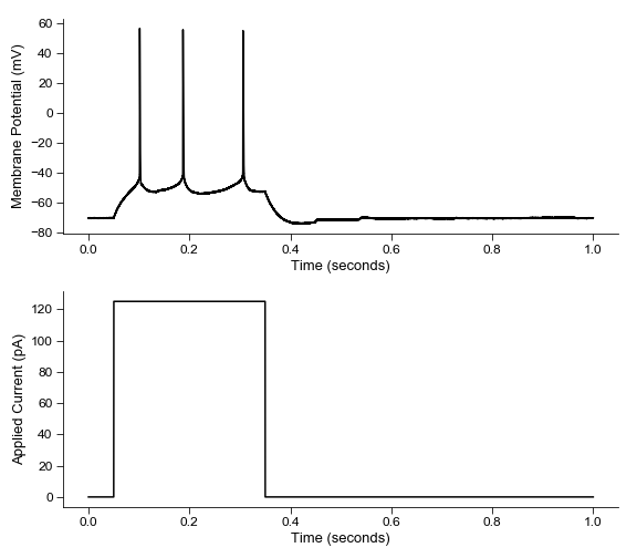
fig = plt.figure(figsize=(8, 7))
ax1 = fig.add_subplot(211)
ax1 = ibt.plot_sweep(sweep_num=16, ax=ax1)

ax2 = fig.add_subplot(212)
ax2 = ibt.plot_command(sweep_num=16, ax=ax2)
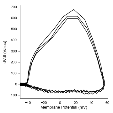
fig = plt.figure(figsize=(5, 5))
ax=ibt.plot_sweep_phase_plane(sweep_num=16)
ax.set_xlim(-50, 60)
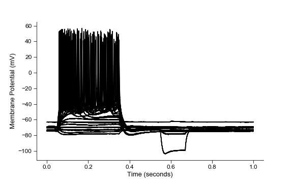
fig=plt.figure(figsize=(8,5))
ax=ibt.plot_all_sweeps()
Get Creative
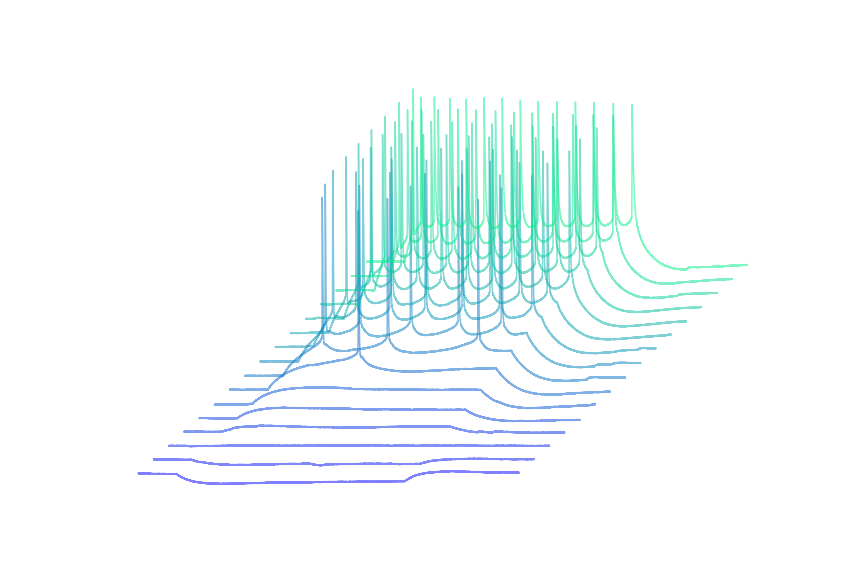
sweeps = ibt.sweeps[9:25]
cm = plt.get_cmap("winter")
colors = [cm(i/len(sweeps)) for i, x in enumerate(sweeps)]

plt.figure(figsize=(12, 8))
for i, sweep in enumerate(sweeps):
    num_pnts = int(0.5/sweep.dx)
    x = sweep.time[:num_pnts] + 0.02 * i
    y = sweep.data[:num_pnts] + 10 * i
    plt.plot(x, y, color=colors[i], alpha=0.5)
plt.gca().axis('off')
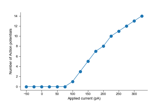
Automatic detection of action potentials
command = 4
sweeps = ibt.sweeps[9:25]

num_APs = []
current = []
for sweep  in sweeps:
    num_APs.append(len(sweep.spike_times_during_command(command)))
    current.append(sweep.commands[4]['value'])

fig=plt.figure(figsize=(8, 5))
plt.plot(current, num_APs, '-o', markersize=10)
plt.ylabel('Number of Action potentials')
plt.xlabel('Applied current (pA)')
plt.savefig('example_plots/FI_curve.png')
import numpy as np

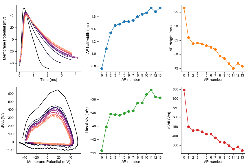
sweep = ibt.sweeps[25]
spikes = sweep.spike_properties()

spike_num = [x for x in range(len(spikes))]
spike_height = [spike['height'] for spike in spikes]
spike_width = [spike['half_width'] for spike in spikes]
spike_thresh = [spike['thresh'] for spike in spikes]
spike_dVdt = [spike['peak_dVdt'] for spike in spikes]

fig = plt.figure(figsize=(12, 8))

ax1 = fig.add_subplot(231)
ax1.set_ylabel('Membrane Potential (mV)')
ax1.set_xlabel('Time (ms)')

ax4 = fig.add_subplot(234)
ax4.set_ylabel('dVdt (V/s')
ax4.set_xlabel('Membrane Potential (mV)')

cm=plt.cm.magma
colors = [cm(i/len(sweeps)) for i, x in enumerate(sweeps)]
for i, spike in enumerate(spikes):
    ax1.plot(spike['time'] * 1000, spike['Vm'], color=colors[i])

    dVdt = np.gradient(spike['Vm'], spike['time'])/1000
    ax4.plot(spike['Vm'], dVdt, color=colors[i])

ax2 = fig.add_subplot(232)
ax2.set_ylabel('AP half width (ms)')
ax2.set_xlabel('AP number')
ax2.set_xticks(spike_num)
ax2.plot(spike_num,spike_width, '-o', markersize=8, color='tab:blue')

ax3 = fig.add_subplot(233, sharex=ax2)
ax3.set_ylabel('AP Height (mV)')
ax3.set_xlabel('AP number')
ax3.plot(spike_num,spike_height, '-o', markersize=8, color='tab:orange')

ax2 = fig.add_subplot(235, sharex=ax2)
ax2.set_ylabel('Threshold (mV)')
ax2.set_xlabel('AP number')
ax2.plot(spike_num,spike_thresh, '-o', markersize=8, color='tab:green')

ax3 = fig.add_subplot(236, sharex=ax2)
ax3.set_ylabel('dVdt (V/s)')
ax3.set_xlabel('AP number')
ax3.plot(spike_num,spike_dVdt, '-o', markersize=8, color='tab:red')
Details of the ibt file structure can be found here
pyibt was inspired by the pyABF module written by Scott Harden for Axon Binary Format (ABF) files.
Author
Perry Spratt
PhD Candidate, Bender Lab
University of California, San Francisco
perrywespratt@gmail.com
Project details
Release history Release notifications | RSS feed
Download files
Download the file for your platform. If you're not sure which to choose, learn more about installing packages.
Source Distribution
Built Distribution
Filter files by name, interpreter, ABI, and platform.
If you're not sure about the file name format, learn more about wheel file names.
Copy a direct link to the current filters
File details
Details for the file pyibt-0.0.2.tar.gz.
File metadata
- Download URL: pyibt-0.0.2.tar.gz
- Upload date:
- Size: 11.7 kB
- Tags: Source
- Uploaded using Trusted Publishing? No
- Uploaded via: twine/3.1.1 pkginfo/1.5.0.1 requests/2.22.0 setuptools/45.0.0 requests-toolbelt/0.9.1 tqdm/4.41.1 CPython/3.6.4
File hashes
| Algorithm | Hash digest | |
|---|---|---|
| SHA256 |
a36b4b77cd3b8357ccf32d1e4d765aadbb352424d53e8464b8d33565ecdeeafa
|
|
| MD5 |
318feaae8caa629ec225b35051b3904d
|
|
| BLAKE2b-256 |
78e0e62fc511b852371c6964afbdafd72100e387e27eefcfa4813c9519f627c6
|
File details
Details for the file pyibt-0.0.2-py3-none-any.whl.
File metadata
- Download URL: pyibt-0.0.2-py3-none-any.whl
- Upload date:
- Size: 10.9 kB
- Tags: Python 3
- Uploaded using Trusted Publishing? No
- Uploaded via: twine/3.1.1 pkginfo/1.5.0.1 requests/2.22.0 setuptools/45.0.0 requests-toolbelt/0.9.1 tqdm/4.41.1 CPython/3.6.4
File hashes
| Algorithm | Hash digest | |
|---|---|---|
| SHA256 |
99c403bfca81d43cf8ea5ba35c632c4d94e973b5ed9a8c083f5ea710b7dc0bd7
|
|
| MD5 |
d607c70b3aa2124154757350903ec29e
|
|
| BLAKE2b-256 |
708f787b3f2e6d09591deea36c9bd6782b6a7b4d1734cbd8a95cc03c100841a0
|


