A Land-Use-Change Cost-Benefit-Analysis calculator coded in Python27&3, PyLUCCBA.

Project description
PyLUCCBA
A Land-Use-Change Cost-Benefit-Analysis calculator coded in Python.
This package offers a compilation of environmental and economic data to generate environment-related net present values of any biofuel project with impacts to the environment (GHG emissions or sequestrations). It is coded in Python (compatible with both versions: 2 and 3). Python is a cross platform and a comprehensive extensible and editable language with a large community of users. The structure of the package is simple with accessible input data to which it is possible to add or suppress one’s own trajectories (of prices, carbon stocks, etc).
NB: In the following description we use the expression project's Net Present Value (NPV) multiple times. Note that this use is abusive since it actually refers to the environmental component of projects. For more details, see Dupoux (In press)
- Code coverage
- Installation
- Example usage
- Invoking documentation
- Data
- Data customization/addition
- Format of results
- Paper's results replication
- References
Code coverage
| Module | statements | missing | excluded | coverage |
|---|---|---|---|---|
| core.py | 880 | 26 | 0 | 97% |
| tools.py | 308 | 60 | 0 | 81% |
| Total | 1188 | 86 | 0 | 93% |
Installation
First, you need Python installed, either Python2.7.+ or Python3.+. Either versions are good for our purpose. Then, we are going to use a package management system to install PyLUCCBA, namely pip, already installed if you are using Python 2 >=2.7.9 or Python 3 >=3.4. Open a session in your OS shell prompt and type
pip install pyluccba
Or using a non-python-builtin approach, namely git,
git clone git://github.com/lfaucheux/PyLUCCBA.git
cd PyLUCCBA
python setup.py install
Example usage
The example that follows is done with the idea of showing how to go beyond the replication of the results presented in Dupoux (In press) via the Python Shell.
Let's first import the module PyLUCCBA
>>> import PyLUCCBA as cc
The alias of PyLUCCBA, namely cc, actually contains many objects definitions, such as that of the calculator that we are going to use in examples. The name of the calculator is CBACalculator.
But before using the calculator as such, let's define (and introduce) the set of parameters that we are going to use to configure CBACalculator. As can be expected when performing a cost benefit analysis, these parameters are related to: (i) the horizon of the project, (ii) the discount rate that we want to use in our calculations, (iii) the scenarized price trajectory of carbon dioxide (CO2), (iv) the scenarized trajectory of quantities of bio-ethanol to produce annually and (...) so on. Let's introduce them all in practice:
>>> cba = cc.CBACalculator(
        run_name               = 'Example-1',
        country                = 'france',
        project_first_year     = 2020,
        project_horizon        = 20,
        discount_rate          = .03,
        co2_prices_scenario    = 'SPC2009',
        output_flows_scenario  = 'O',
        initial_landuse        = 'improved grassland',
        final_landuse          = 'wheat',
        input_flows_scenario   = 'IFP',
        T_so                   = 20,
        T_vg_diff              = 1,
        T_vg_unif              = 20,
        polat_repeated_pattern = True,
        final_currency         = 'EUR',
        change_rates           = {'EUR':{'USD/EUR':1.14}}, # https://www.google.fr/#q=EUR+USD
        return_charts          = True,
        save_charts            = True,
        from_local_data        = False,
    )
The following table enumerates all parameters that can be used to create an instance of CBACalculator.
| Parameter's name | Description |
|---|---|
run_name |
name of the folder that will contain the generated results and charts, e.g. 'Example-1'. |
country |
name of the country under study. Only one possible choice currently: France. |
project_first_year |
first year of the project. |
project_horizon |
duration of the biofuel production project (years). |
discount_rate |
rate involved in the calculations of net present values. Set to 0. by default. |
co2_prices_scenario |
name of the trajectory of CO2 prices. The current choices are 'A', 'B', 'C', 'DEBUG', 'O', 'OECD2018', 'SPC2009', 'SPC2019', 'WEO2015-450S', 'WEO2015-CPS', 'WEO2018-CPS', 'WEO2015-NPS', 'WEO2018-NPS' or 'WEO2018-SDS'. |
output |
name of the produced biofuel. Set to 'eth' by default. Only one possible choice currently: 'eth'. NB: 'eth' actually stands for bioethanol. |
black_output |
name of the counterfactual produced output. Serves as the reference according to which the production of bioethanol ('eth') is considered (or not) as pro-environmental. Set to 'oil' by default. Only one possible choice currently: 'oil'. NB: 'oil' actually stands for gasoline. |
output_flows_scenario |
name of the trajectory of annually produced quantities of biofuel. The current choices are 'DEBUG' or 'O'. |
initial_landuse |
use of the land before land conversion. The current choices are 'forestland30', 'improved grassland', 'annual cropland' or 'degraded grassland'. |
final_landuse |
use of the land after land conversion. The current choices are 'miscanthus', 'sugarbeet' or 'wheat'. |
input_flows_scenario |
name of the trajectory of input-to-ouput yields. The current choices depend on the value set for final_landuse. If final_landuse is set to 'miscanthus', the possibilities are 'DEBUG' and 'DOE'. If final_landuse is set to 'wheat' or 'sugarbeet', the possibilities are 'IFP' and 'DEBUG'. |
T_so |
period over which soil carbon emissions due to LUC are considered. |
T_vg_diff |
period over which vegetation carbon emissions due to LUC are considered in the differentiated annualization approach. |
T_vg_unif |
period over which vegetation carbon emissions due to LUC are considered in the uniform annualization approach. |
polat_repeated_pattern |
if True, retro/extra-polation pattern is repeated before/after the first/last mentioned value. Otherwise, it is maintained constant. |
final_currency |
currency used to conduct the study and express the results. The current choices are 'EUR' or 'USD'. Set to 'EUR' by default. |
change_rates |
final_currency-dependent exchange rate to consider in calculations, e.g. {'EUR':{'USD/EUR':1.14,}} (or {'EUR':{'EUR/USD':0.8772,}} since the tool ensures dimensional homogeneity). |
return_charts |
if True, charts are returned (for interactive use, e.g. hovering). Set to True by default. |
save_charts |
if True, charts are saved on the disk. Set to True by default. |
from_local_data |
if True, scenarized trajectories (e.g. of CO2 prices, of output flows quantities, of yields) are read from the 'resources' folder that is located next to the working script. If False, those are read from the 'resources' folder natively contained in the package directory. Set to False by default. |
Once we have our instance of CBACalculator in hand, i.e. cba, we may wonder what are the scenarized trajectories over which we are about to conduct our study, e.g. of CO2 prices, produced quantities of biofuel, etc. In this case, we can simply type:
>>> cba.chart_of_output_flows_traj.show()
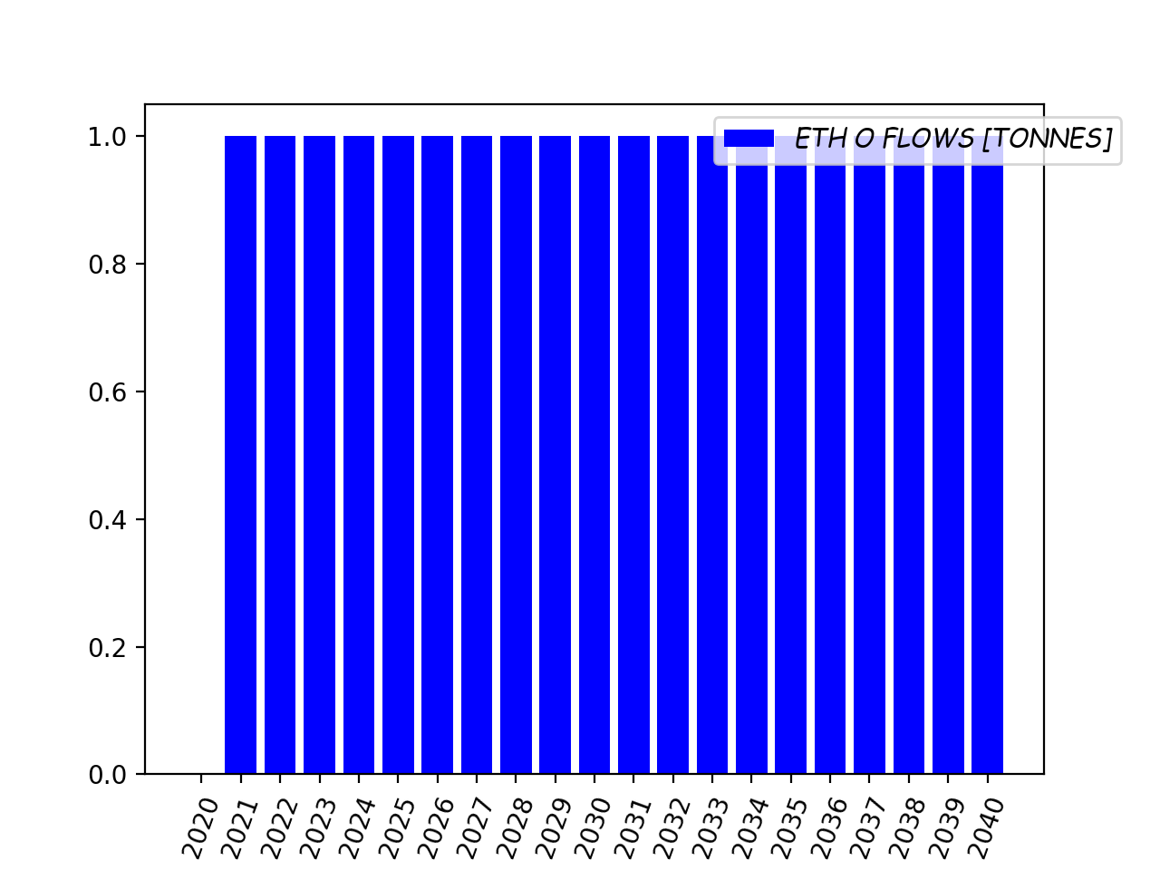
As it reads in the above chart, we are about to work with a constant level of production over the project horizon. Note the absence of flow in 2020: this illustrates the need for waiting one year before having enough wheat to produce biofuel.
We may then wonder what is the counterfactual trajectory in terms of gasoline – targeting the same energy efficiency (in joule) as conversion basis:
>>> cba.chart_of_black_output_flows_traj.show()

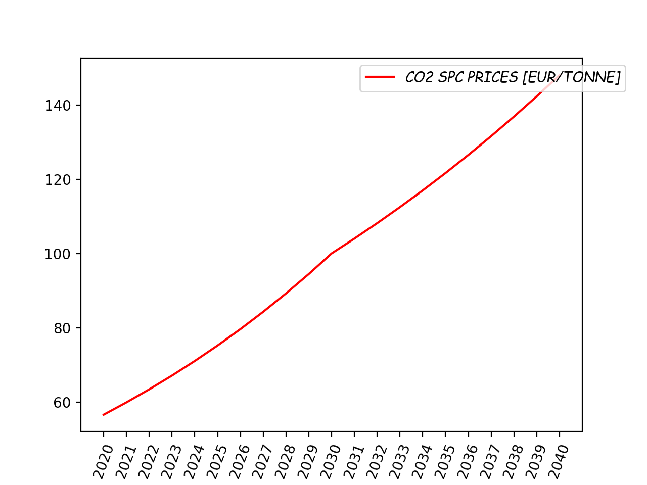
Now, let's see which trajectory of CO2 prices is behind the name 'SPC2009' – which stands for Quinet (2009)'s shadow price of carbon:
>>> cba.chart_of_co2_prices_traj.show()
We may also wonder which quantities trajectory of wheat is implied by that of biofuel on the one hand, and by the value we set for the parameter input_flows_scenario, that is 'IFP' , on the other hand – where I.F.P stands for Institut Français du Pétrole énergies nouvelles – which made a report in 2013 in which it reads that, with 1 tonne of wheat, one can produce 0.2844 tonnes of bioethanol. Let's vizualize that:
>>> cba.chart_of_input_flows_traj.show()
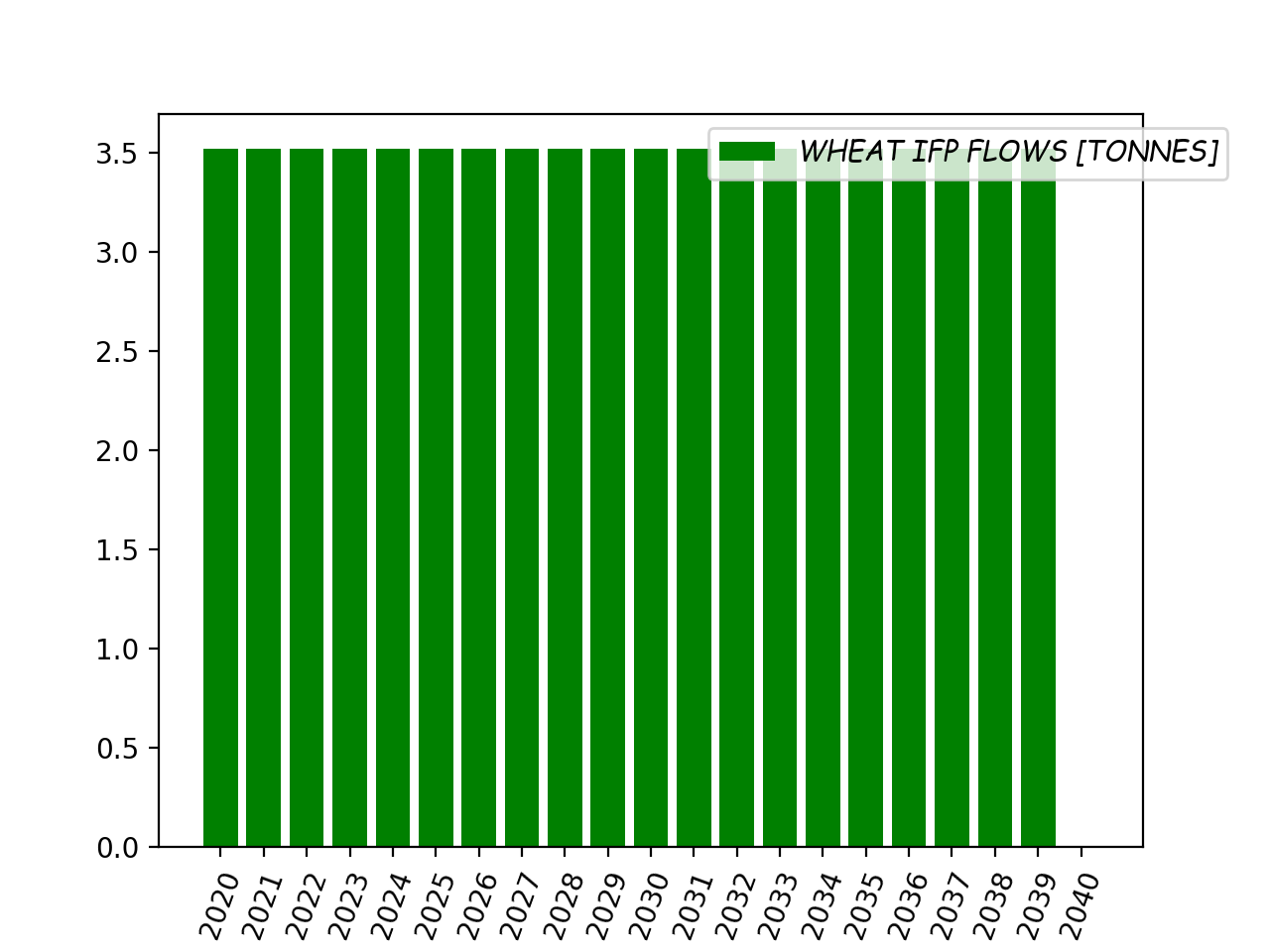
Note the absence of input flow in 2040: as explained previously, this illustrates the time delay that exists between the cultivation of wheat and its processing into bioethanol, e.g. wheat cultivated in 2039 is used for the production of bioethanol planned in 2040.
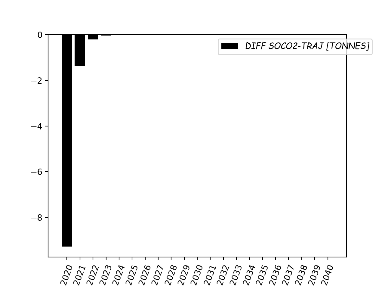
The land use change from initial_landuse='improved grassland' to final_landuse='wheat' has effects in terms of CO2 emissions. These emissions clearly do not exhibit the same profile depending on how we choose to consider them over the project horizon. First, regarding soil CO2 emissions:
>>> cba.carbon_and_co2_flows_traj_annualizer.so_emitting
True
>>> cba.chart_of_soco2_unif_flows_traj.show()
>>> cba.chart_of_soco2_diff_flows_traj.show()
---- a_parameter_which_solves_soc_chosen_CRF_constrained sol=[0.52418009]
---- [***]The solution converged.[0.000000e+00][***]

Of course, the comparison makes sense since the total emitted stocks are identical:
>>> import numpy as np
>>> np.sum(cba.soco2_unif_flows_traj)
-10.90041830757967 # tonnes
>>> np.sum(cba.soco2_diff_flows_traj)
-10.90041830757967 # tonnes
On the side of vegetation-related emissions, converting grassland into wheat field generates a loss of carbon since the latter is harvested annually while the former sequestrates carbon on a pertpetual basis. Here again, emissions' profiles are clearly different under differentiated or uniform annualization approach, see
>>> cba.carbon_and_co2_flows_traj_annualizer.vg_emitting
True
>>> cba.chart_of_vgco2_unif_flows_traj.show()
>>> np.sum(cba.vgco2_unif_flows_traj)
-7.130970463238133 # tonnes
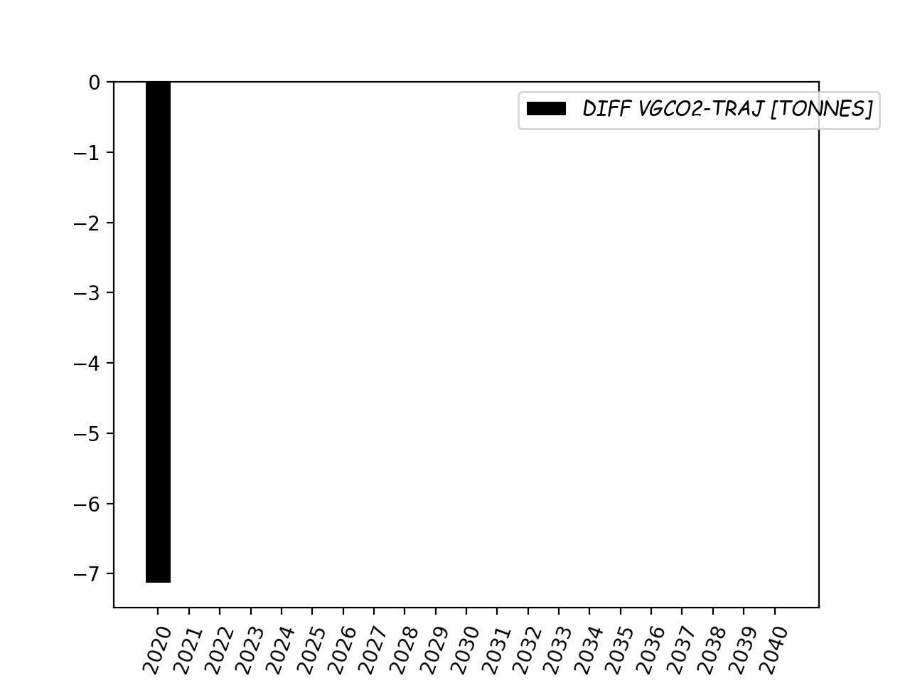
>>> cba.chart_of_vgco2_diff_flows_traj.show()
---- a_parameter_which_solves_vgc_chosen_CRF_constrained sol=[0.02458071]
---- [***]The solution converged.[0.000000e+00][***]
>>> np.sum(cba.vgco2_diff_flows_traj)
-7.130970463238132 # tonnes

Independently of how we annualize the LUC-related CO2 emissions, the cultivation and the processing of wheat generate emissions annually as well. See
>>> cba.chart_of_cult_input_co2eq_flows_traj.show()
>>> cba.chart_of_proc_input_co2eq_flows_traj.show()
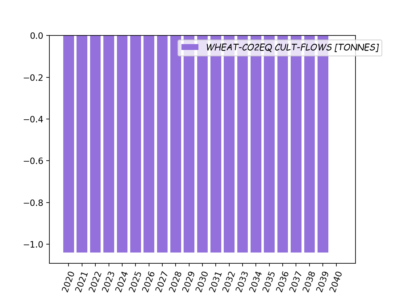
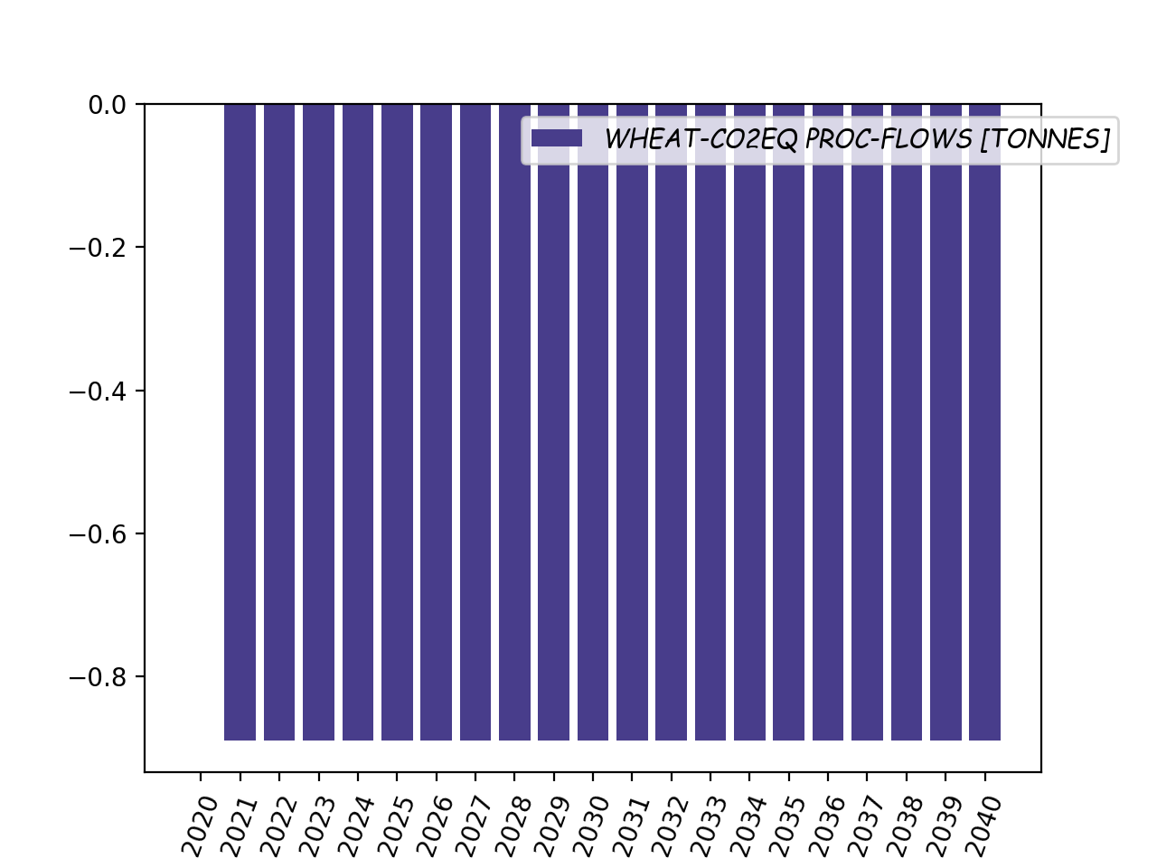
Once again, the two above charts unambiguously illustrate the time delay that exists between the cultivation of wheat and its processing into bioethanol, i.e. wheat cultivated in year t-1 is used for the production of bioethanol planned in year t. Also, note that these cultivation- and processing-related emissions are in CO2eq since CH4 and N2O flows are considered as well, using their relative global warming potentials – relatively to that of CO2 – as a basis of conversion. See calculation details at PyGWP.
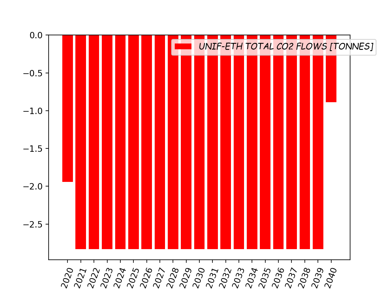
Finally, under the two types of annualization approach, the total emissions following a change in land use from improved grassland into wheat field are:
>>> cba.chart_of_total_unif_co2_flows_traj.show()
>>> cba.chart_of_total_diff_co2_flows_traj.show()
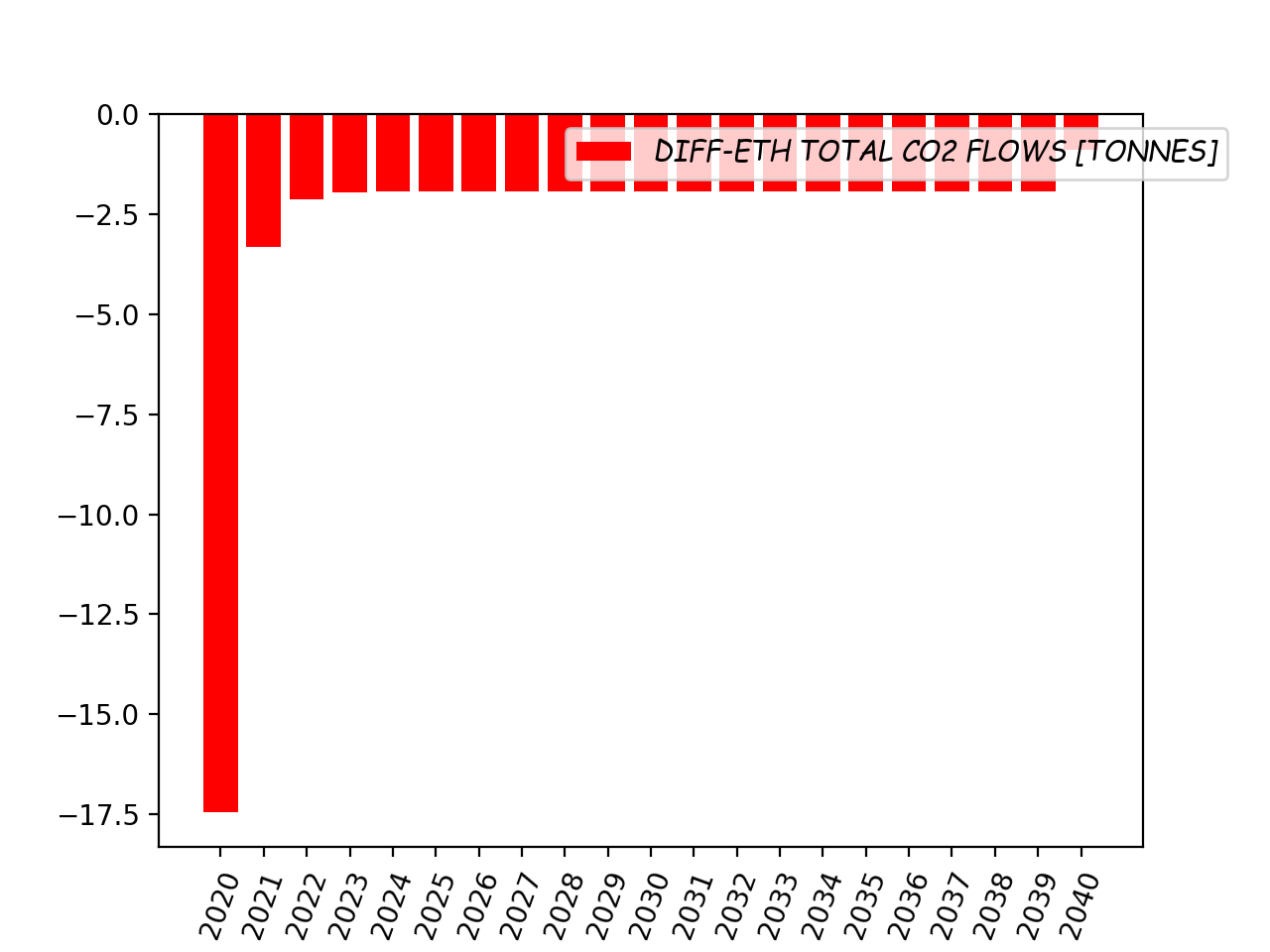
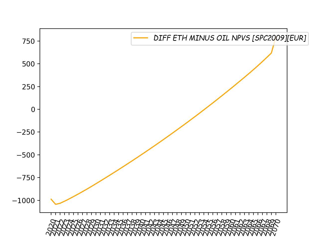
which, when monetized with a non-zero discount rate and compared in terms of absolute deviations from gasoline's valorized CO2 flows, lead to sensitivly different profiles for the values of the environmental component of the project, see rather
>>> cba.chart_of_NPV_total_unif_minus_black_output_co2_flows_trajs.show()
>>> cba.chart_of_NPV_total_diff_minus_black_output_co2_flows_trajs.show()
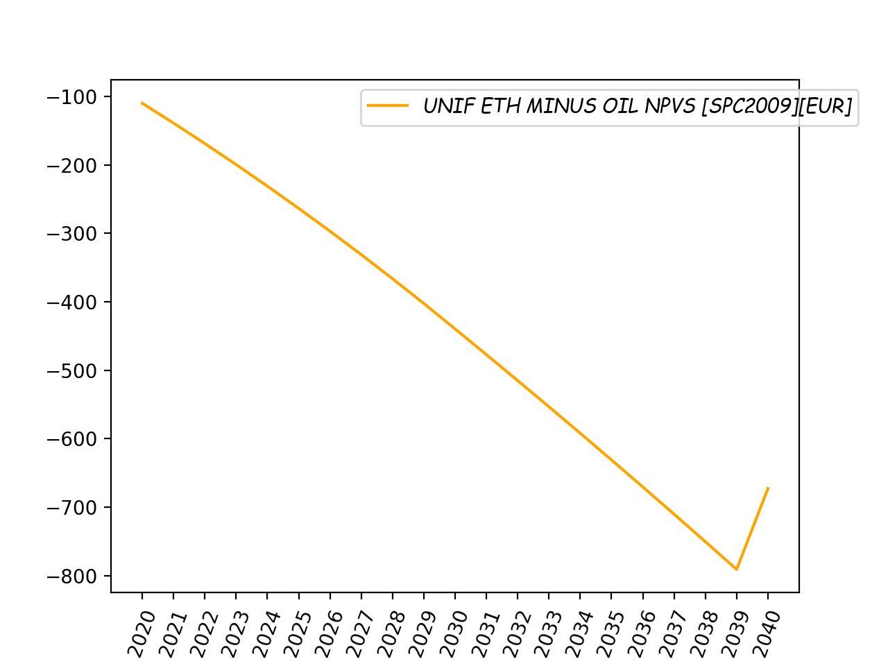
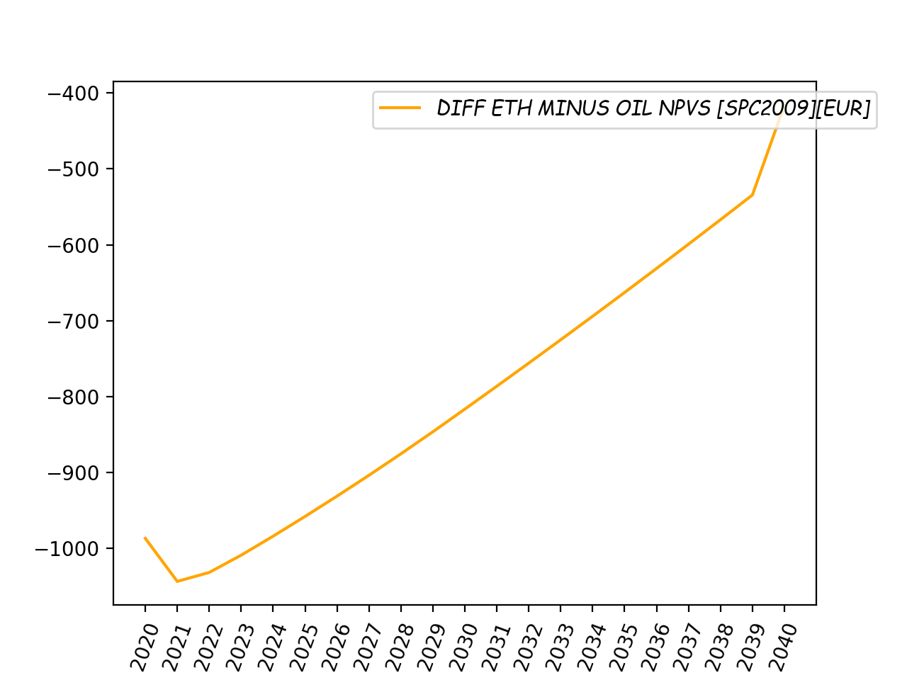
Note the slope-breaks that occur during the last year. This is due to the fact that cultivation and its associated emission flows generally – depending on the type of final land use – finish one year before the end of the project, which structurally increases projects' NPVs.
A note on the carbon profitability payback period
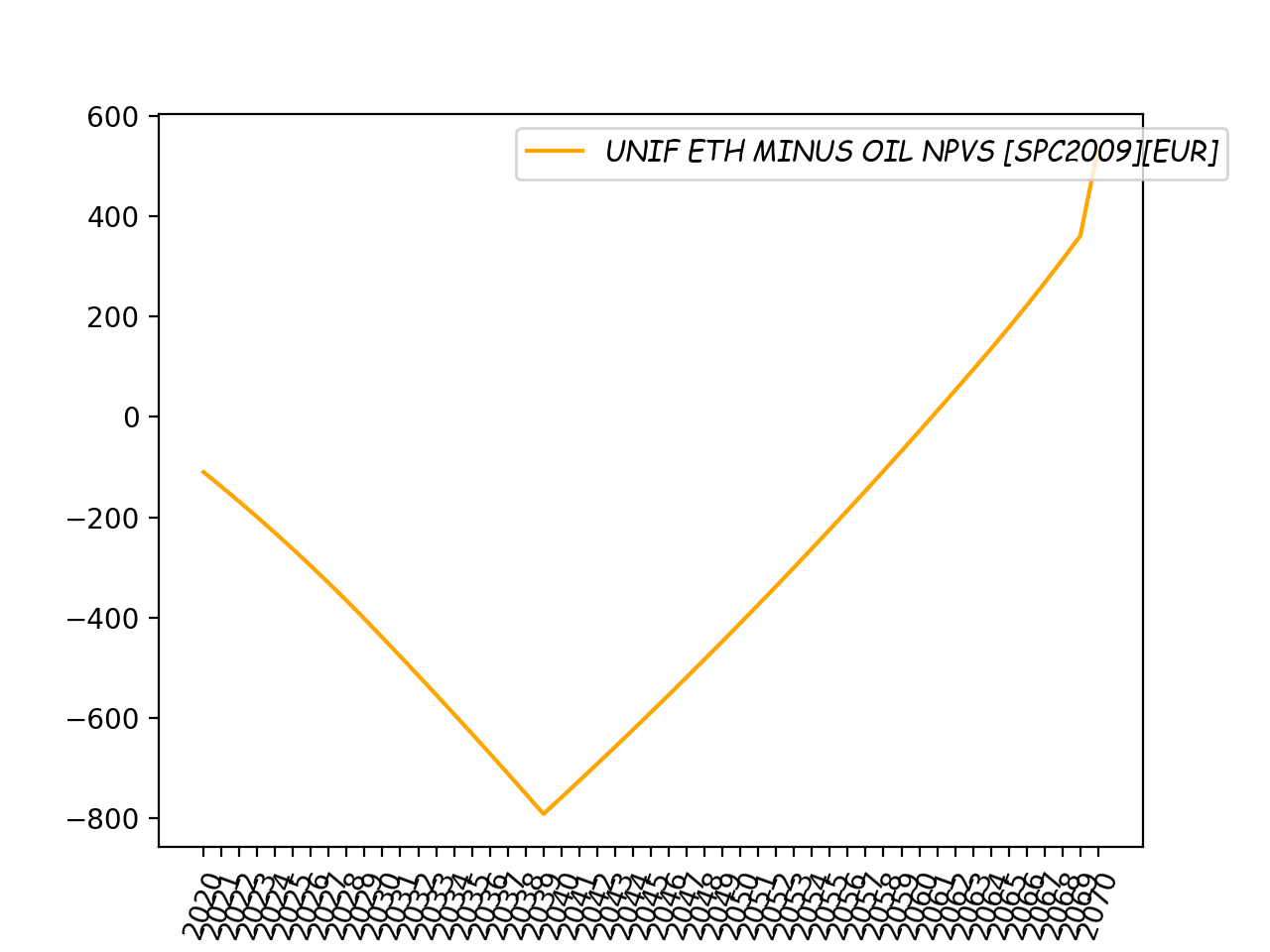
Actually, it looks like extending the horizon of the project may be a good idea to see whether one of the two NPVs' profiles – shown above – exhibit positive values over the long run. Put differently, let's vizualize when the project exhibits positive NPV under each annualization approach.
• NB1: the project horizon must be long enough for such a payback period to exist. Hence the extension from 20 to 50 years configured below.
• NB2: given that cultivation and its associated flows of emission generally – depending on the type of final land use – stop before the end of the project, the last year of the project is structurally more environment-friendly, which increases projects' NPVs (see the jump in the charts above), in some cases to such an extent that the last year actually becomes the payback period, hence the NB1.
>>> cba._clear_caches()    # we clear the cache of our instance since we are going to change a calculation parameter.
GlobalWarmingPotential     # the tool enumerates objects whose cache have been cleaned.
OutputFlows
CarbonAndCo2FlowsAnnualizer
LandSurfaceFlows
Co2Prices
CBACalculator
>>> cba.project_horizon = 50    # we set a long project horizon
>>> cba.chart_of_NPV_total_unif_minus_black_output_co2_flows_trajs.show()
>>> cba.chart_of_NPV_total_diff_minus_black_output_co2_flows_trajs.show()
---- a_parameter_which_solves_soc_chosen_CRF_constrained sol=[0.52418009]
---- [***]The solution converged.[0.000000e+00][***]
---- a_parameter_which_solves_vgc_chosen_CRF_constrained sol=[0.02458071]
---- [***]The solution converged.[0.000000e+00][***]
Rather than vizualizing the NPVs' profiles, we may use a precise way to know when a project becomes environmentally profitable – referred to as Carbon Profitability Payback Period in Dupoux (In press) – for each type of annualization approach.
>>> cba.unif_payback_period
41 # years
>>> cba.diff_payback_period
35 # years
Let's be precautious and go back to the project's settings of interest for the rest of the example.
>>> cba._clear_caches()
GlobalWarmingPotential
OutputFlows
CarbonAndCo2FlowsAnnualizer
LandSurfaceFlows
Co2Prices
CBACalculator
>>> cba.project_horizon = 20    # let's go back to our initial settings !
A note on the compensatory rate
We may wonder under which discount rate the two approaches of annualization – uniform versus differentiated – would lead to the same NPV over the project horizon. To do so, we have to use another object that is defined in PyLUCCBA, namely CBAParametersEndogenizer. Let's continue our example and instantiate it:
>>> gen = cc.CBAParametersEndogenizer(CBACalculator_instance = cba)
With gen in hand, we can now determine which discount rate equalizes our two NPVs, as follows:
>>> cba_eq = gen.endo_disc_rate_which_eqs_NPV_total_unif_co2_flows_traj_to_NPV_total_diff_co2_flows_traj
---- a_parameter_which_solves_soc_chosen_CRF_constrained sol=[0.52418009]
---- [***]The solution converged.[0.000000e+00][***]
---- a_parameter_which_solves_vgc_chosen_CRF_constrained sol=[0.02458071]
---- [***]The solution converged.[0.000000e+00][***]
---- disc rate equating unif- and diff-based NPVs sol=[0.05420086]
---- [***]The solution converged.[4.440892e-16][***]
Note that cba_eq is the disc_rate-balanced counterpart of cba. It reads above that, "so configured", our project would have identical NPVs under the uniform and differentiated annualization approaches for a discount rate of 5.42%.
At anytime, we can have a quick look at what is meant exactly by "so configured", typing
>>> print(cba_eq.summary_args)
**************************************************************************************
run_name                : Example-1
output                  : ETH
black_output            : OIL
initial_landuse         : IMPROVED GRASSLAND
final_landuse/input     : WHEAT
country                 : FRANCE
project_horizon         : 21 # because of the time delay between cultivation and processing, taken at t0 - 1.
T_so                    : 20
T_vg_diff               : 1
T_vg_unif               : 20
project_first_year      : 2020
polat_repeated_pattern  : True
co2_prices_scenario     : SPC2009
discount_rate           : [0.05420086] # our endogenized compensatory rate
diff_payback_period     : []
unif_payback_period     : []
final_currency          : EUR
change_rates            : {'USD/EUR': 1.14}
output_flows_scenario   : O
input_flows_scenario    : IFP
message                 : _ENDOGENIZER finally says sol=0.0542008612895724
                          obj(sol)=[4.4408921e-16]
Invoking documentation
You should abuse of the python-builtin function help on any object defined in PyLUCCBA, as well as on any instantiated object, e.g.
>>> import PyLUCCBA as cc
>>> help(cc.CBAParametersEndogenizer)
Help on CBAParametersEndogenizer in module PyLUCCBA.core object:

class CBAParametersEndogenizer(builtins.object)
 |  Class object designed to handle a CBACalculator instances and to
 |  endogenize some of its parameter.
 |
 |  Methods defined here:
 |
 |  __init__(self, CBACalculator_instance)
 |      Initialize self.  See help(type(self)) for accurate signature.
 |
 |  ----------------------------------------------------------------------
 |  Data descriptors defined here:
 |
 |  OBJECTIVE_NPV_total_unif_co2_flows_traj_VS_NPV_total_diff_co2_flows_traj
 |      Method which computes the objective of the discount rate
 |      endogenizing process.
 |
 |      Testing/Example
 |      ---------------
 |      >>> _dr_ = 0.03847487575799428 ## the solution
 |      >>> cba = CBACalculator._testing_instancer(
 |      ...     dr = _dr_,
 |      ...     sc = 'WEO2015-CPS',
 |      ... )
 |      >>> CBAParametersEndogenizer(
 |      ...     CBACalculator_instance = cba
 |      ... ).OBJECTIVE_NPV_total_unif_co2_flows_traj_VS_NPV_total_diff_co2_flows_traj
 |      ---- a_parameter_which_solves_soc_chosen_CRF_constrained sol=[0.52418009]
 |      ---- [***]The solution converged.[0.000000e+00][***]
 |      ---- a_parameter_which_solves_vgc_chosen_CRF_constrained sol=[0.02458071]
 |      ---- [***]The solution converged.[0.000000e+00][***]
 |      array([2.22044605e-16])
 |
 |  __dict__
 |      dictionary for instance variables (if defined)
 |
 |  __weakref__
 |      list of weak references to the object (if defined)
 |
 |  endo_disc_rate_which_eqs_NPV_total_unif_co2_flows_traj_to_NPV_total_diff_co2_flows_traj
 |      Returns a CBACalculator instance configured with the discount rate
 |      which equates NPV_total_unif_co2_flows_traj TO NPV_total_diff_co2_flows_traj.
 |
 |      Testing/Example
 |      ---------------
 |      >>> cba = CBACalculator._testing_instancer(
 |      ...     sc = 'WEO2015-CPS',
 |      ... )
 |      >>> o = CBAParametersEndogenizer(
 |      ...     CBACalculator_instance = cba
 |      ... )
 |      >>> o.endo_disc_rate_which_eqs_NPV_total_unif_co2_flows_traj_to_NPV_total_diff_co2_flows_traj.discount_rate[0]
 |      ---- a_parameter_which_solves_soc_chosen_CRF_constrained sol=[0.52418009]
 |      ---- [***]The solution converged.[0.000000e+00][***]
 |      ---- a_parameter_which_solves_vgc_chosen_CRF_constrained sol=[0.02458071]
 |      ---- [***]The solution converged.[0.000000e+00][***]
 |      ---- disc rate equating unif- and diff-based NPVs sol=[0.03847488]
 |      ---- [***]The solution converged.[2.220446e-16][***]
 |      0.038474875757994256
I invite you to test the function help on any of the following objects: cc.BlackOutputAndSubstitutesSpecificities, cc.CBACalculator, cc.CBAParametersEndogenizer, cc.CarbonAndCo2FlowsAnnualizer, cc.Co2Prices, cc.GlobalWarmingPotential, cc.InputFlows, cc.LandSurfaceFlows, cc.OutputFlows, cc.VGCAndSOCDeltas, cc.VegetationsAndSoilSpecificities.
Data
Data are stored in the resources folder, composed of the following subfolders:
• The meta folder, which includes BioGrace Excel tool - version 4c.xls and Data_CarbonStocks_Emissions.xlsx, in which you can see all the calculations of carbon stocks for each type of land use.
• The dluc folder, which includes three datafiles, namely (i) cs_changes_fr.csv relating to the carbon stock associated with specific types of land use, (ii) so_ghgs_shares_fr.csv relating to the share of soil carbon that translate to actual emissions/sequestrations and (iii) vg_ghgs_shares_fr.csv relating to the share of vegetation carbon that translate to actual emissions/sequestrations. Each of these csv files possesses a txt counterpart with the same name, which provides mandatory information regarding, e.g., the unit of measurement of data.
• The externality folder, which includes three datafiles, namely (i) co2_prices_fr.csv relating to the CO2 price-trajectory scenarios, (ii) cult_ghgs_fr.csv relating to the quantity of GHG emissions associated with the cultivation of land and (iii) proc_ghgs_fr.csv relating to the processing of energy crop to biofuel. Each of these csv files possesses a txt counterpart that has the same name, which provides mandatory information regarding, e.g., the unit of measurement of data.
• The input folder, which includes four datafiles, namely (i) haeth_yields_fr.csv relating to the number of tonnes of ethanol per hectare over time and (ii) miscanthus_yields_fr.csv, sugarbeet_yields_fr.csv and wheat_yields_fr.csv relating to the number of tonnes of feedstock necessary to produce one tonne of biofuel. As before, almost each of these csv files has a txt counterpart that provides mandatory information on data. In the case of datafiles with no txt counterpart, the tool searches for information in a txt file with the same name as the parent folder's, i.e. input.txt in this case.
• The output folder, which includes three datafiles, namely (i) eth_yields_fr.csv that tautologically states that one tonne of biofuel is produced per tonne of output, (ii) cult_to_proc_delays_fr.csv relating to the time delay required between cultivation and processing of feedstock and (iii) subs_intensities_fr.csv relating to the amount of energy and emissions associated with bioethanol and oil. Once again, each of these csv files has a txt counterpart that provides mandatory information on data.
NB1: all files with a name containing either "_yields" or "_prices" consist of temporal trajectories. These trajectories can be sparse. Indeed, when sparse trajectories with more than one point are provided, say, CO2 prices such as in the scenario WEO2015-CPS – see co2_prices_fr.csv –, the tool automatically retro/inter/extrapolates the values for each year in an exponential way. When both retro- and extrapolation are possible, retropolation is chosen by using the next period's rate of growth. Then, if the parameter polat_repeated_pattern is set to True, extrapolation is performed by repeating the entire anterior pattern of growth rates from the last known value. If the parameter is set to False, the last known value is kept constant over the project horizon. In the case of sparse trajectories that contain only one value – see e.g. wheat_yields_fr.csv –, the trajectory is assumed to be flat over the project horizon.
NB2: all files with a name containing either "_yields" or "_prices" must possess a txt file counterpart providing information on their unit of measurement. Indeed, they are read and interpreted with the intention of ensuring the dimensional homogenity of calculations. For example, if, say, tonne/ha is required for calculation and that the unit of measurement is ha/tonne, the numerical inverse is computed prior to core-calculations.
Data customization/addition
You may want to add your own scenarii regarding, e.g., how the price of CO2 evolves over time, the trajectory of output flows produced annually, the quantity of input that is required to produce 1 tonne of output, etc... The easiest way of working with custom data is to imitate the package-native data contained in the resources folder. Let's start with a local copy of this folder:
>>> import PyLUCCBA as cc
>>> cc.folder_copier(name='resources')
'resources' folder copied to C:\path\to\folder
Now, to explore the data, go to C:\path\to\folder, where you will see a folder named resources that is the exact copy of the data used in Dupoux (In press).
Adding new data
To add new data, e.g. a scenario of CO2 prices, go to the folder resources\externality of your local copy. There, you will find two files, namely co2_prices_fr.csv and co2_prices_fr.txt. First, open the csv file, add a scenario's name in the first line, e.g. customPricesScenario, and prices in the just-named column. Remember that your newly-added trajectory can be sparse and that the tool will retro/intra/extrapolate missing prices. Second, open the txt file and add two lines related to customPricesScenario, as shown below:
customPricesScenario:unit:EUR/tonne
customPricesScenario:yrb:none
The first line specifies the currency in which prices are expressed. Note that the tool is actually not capable of dealing with other mass-units than tonne, so stick to it. The second line is not mandatory. It only allows you to simplify the potential future improvements of the tool. Finally, to imply the just-added trajectory of prices in your calculations, simply instantiate CBACalculator with 'customPricesScenario', i.e.
>>> cba = cc.CBACalculator(
        # ...
        co2_prices_scenario = 'customPricesScenario', # not case sensitive
        from_local_data     = True, # [!!!]
        # ...
    )
Note that to add a new trajectory of annual output flows or one of yields, the approach is exactly the same as that described for CO2 prices. Simply enrich/modify your local copy.
Format of results
The generated results consist of three .xlsx files, namely _quantities.xlsx, _values.xlsx and _NPVs.xlsx all three located in a folder that is named (by default) according to the arguments involved in the computation:
• _quantities.xlsx displays the quantities associated to each flow, among which, emissions from the process of production, emissions from the cultivation of the feedstock, land use change impact from soil, land use change impact from biomass, etc.
• _values.xlsx displays the monetary value of the different types of flows from both bioethanol and gasoline (“black”) depending of the carbon price scenario that is chosen.
• _NPVs.xlsx displays the net present values for both the uniform and the differentiated annualizations for the different types of flow again.
Note that each column has a title that is very verbose – so as to make things as explicit as possible – regarding what is calculated. When the prefix ut_ appears in the title it means that it is calculated for one unit tonne of biofuel. When the prefix um_ appears in the title, it means that it is calculated for one unit megajoule of biofuel. When nothing is specified, it takes into account the total quantity of biofuel produced.
Paper's results replication
All the results presented in Dupoux (In press) can easily be reproduced. To replicate a specific result, one has to import the associated script. Its importation will run the code that is required to generate the results. The table that follows makes the association between the python import-commands and the cases presented in the paper.
| Paper's section and page | Python command | Invoked script |
|---|---|---|
| Subsection 3.2 page 12 | from PyLUCCBA.examples import study_Grassland_DiscountingEffect |
study_Grassland_DiscountingEffect.py |
| Subsection 3.2 page 13 | from PyLUCCBA.examples import study_Grassland_CarbonPriceEffect |
study_Grassland_CarbonPriceEffect.py |
| Subsection 3.2 page 14 | from PyLUCCBA.examples import study_Grassland_CombinedEffect |
study_Grassland_CombinedEffect.py |
| Subsection 4.1 page 14 | from PyLUCCBA.examples import study_Grassland_CompensatoryRate |
study_Grassland_CompensatoryRate.py |
| Subsection 4.2 page 15 | from PyLUCCBA.examples import study_Grassland_PaybackPeriod |
study_Grassland_PaybackPeriod.py |
In case you want to modify those scripts instead of simply invoking them, you can first copy them to your working directory, typing
>>> import PyLUCCBA as cc
>>> cc.folder_copier(name='examples')
'examples' folder copied to C:\path\to\folder
Second, go to C:\path\to\folder, where you will see a folder named examples that contains the exact copies of the scripts enumerated in the above table. To edit one of those scripts, say, study_Grassland_CompensatoryRate.py, right-click it and select option Edit with IDLE. Modify anything you want. To execute the script, type F5.
References
Hoefnagels, R., E. Smeets, and A. Faaij (2010). “Greenhouse gas footprints of different biofuel production systems”. Renewable and Sustainable Energy Reviews 14.7, pp. 1661–1694.
IEA (2015). World Energy Outlook 2015. Tech. rep. International Energy Agency.
IPCC (2006). “Volume 4: Agriculture, Forestry and Other Land Use”. IPCC guidelines for national greenhouse gas inventories 4.
Poeplau, C., A. Don, L. Vesterdal, J. Leifeld, B. VanWesemael, J. Schumacher, and A. Gensior (2011). “Temporal dynamics of soil organic carbon after land-use change in the temperate zone - carbon response functions as a model approach”. Global Change Biology 17.7, pp. 2415–2427.
The European Commission (2010). “Commission decision of 10 June 2010 on guidelines for the calculation of land carbon stocks for the purpose of Annex V to Directive 2009/28/EC”. Official Journal of The European Union 2010/335/E.
Dupoux, M. “The land use change time-accounting failure” (in press).


Download files
Download the file for your platform. If you're not sure which to choose, learn more about installing packages.
Source Distribution
Built Distribution
Filter files by name, interpreter, ABI, and platform.
If you're not sure about the file name format, learn more about wheel file names.
Copy a direct link to the current filters
File details
Details for the file PyLUCCBA-0.9.23.tar.gz.
File metadata
- Download URL: PyLUCCBA-0.9.23.tar.gz
- Upload date:
- Size: 8.5 MB
- Tags: Source
- Uploaded using Trusted Publishing? No
- Uploaded via: twine/1.12.1 pkginfo/1.5.0.1 requests/2.21.0 setuptools/39.0.1 requests-toolbelt/0.9.1 tqdm/4.31.1 CPython/3.7.1
File hashes
| Algorithm | Hash digest | |
|---|---|---|
| SHA256 |
5301cde4cc01e4bfaac6db4f8d99d4b159aab29ae65266a19b8a8b9d83452245
|
|
| MD5 |
9953d0436eb4e9875757065b6de27579
|
|
| BLAKE2b-256 |
4fe67946249e9eddb869f50be09413e331d7317b34929a3afd24744896c85373
|
File details
Details for the file PyLUCCBA-0.9.23-py2-none-any.whl.
File metadata
- Download URL: PyLUCCBA-0.9.23-py2-none-any.whl
- Upload date:
- Size: 8.8 MB
- Tags: Python 2
- Uploaded using Trusted Publishing? No
- Uploaded via: twine/1.12.1 pkginfo/1.5.0.1 requests/2.21.0 setuptools/39.0.1 requests-toolbelt/0.9.1 tqdm/4.31.1 CPython/3.7.1
File hashes
| Algorithm | Hash digest | |
|---|---|---|
| SHA256 |
3acb9a1497e95ec647d5d1db4b451bf91cd719481fa72d700a6c13d4e26e07c9
|
|
| MD5 |
c6446c1d6a8c6676eb5693eda9b0506c
|
|
| BLAKE2b-256 |
ce1af290215487ab5ef9e79a021f80a7eec3bb002c53a2e3474ca5f682d5c2de
|


