
pynonthermal




pynonthermal is a Python solver for the Spencer-Fano equation. The equation describes the energy distribution of the non-thermal (fast) electrons that slow down in a plasma. Radioactive decay in supernova ejecta makes high-energy leptons: Compton, photoelectric, and pair-production electrons and positrons. A partially ionised gas takes their energy through three channels:
- Coulomb heating of the free thermal electrons;
- collisional ionisation;
- collisional excitation of bound states.
Given a set of ions with number densities and an energy deposition rate, pynonthermal computes:
- the degradation spectrum y(E) of the non-thermal electron population;
- the fraction of the deposited energy that goes to heating, ionisation, and excitation, per channel and per ion;
- the non-thermal ionisation rate coefficients of each ion and the excitation rate coefficients of bound-bound transitions, for non-LTE plasma models.
These quantities are important in models of the late-time spectra and light curves of Type Ia and core-collapse supernovae, where non-thermal ionisation can dominate over photoionisation. The solver follows the method of Kozma and Fransson (1992, ApJ, 390, 602–621, doi:10.1086/171296) (see Method background for details and further references). It includes the atomic data that it needs: ionisation cross sections for a wide range of ions, and level and transition data for bound-bound excitation.
Contents
- Installation
- Quick start
- Usage guide
- Where the ion populations come from
- Complete example: pure-oxygen plasma
- Units and conventions
- Method background
- Cross-section datasets
- Advanced usage: custom cross sections
- Citing pynonthermal
- License
Installation
Released package (recommended for most users):
pip install pynonthermal
Development install with uv:
git clone https://github.com/lukeshingles/pynonthermal.git
cd pynonthermal
uv sync --frozen
source ./.venv/bin/activate
uv pip install --editable .
prek install
Run the test suite with:
uv run -- python3 -m pytest
Quick start
Make a solver, add the elements of the gas, solve, then read the results:
import pynonthermal

with pynonthermal.SpencerFanoSolver() as sf:
    # O II (ion_stage=2, i.e. charge +1) at a number density of 1e8 cm^-3
    sf.add_element(Z=8, ion_densities={2: 1.0e8})

    sf.solve(deposition_ev_per_s_per_cm3=1.0e8)  # the rate of energy deposition per volume

    print("heating fraction:", sf.get_frac_heating())
    print("ionisation fraction:", sf.get_frac_ionisation_tot())
    print("excitation fraction:", sf.get_frac_excitation_tot())
    print("sum of fractions:", sf.get_frac_sum())
    print("ionisation rate coeff [s^-1]:", sf.get_ionisation_ratecoeff(Z=8, ion_stage=2))
The solver is a builder. Each call adds ions, ionisation channels, or excitations to the matrix, and solve()
solves it. The with block is optional and only scopes the solver.
The quickstart notebook contains a fuller worked example. Binder can run it:

Usage guide
1. Make the solver
sf = pynonthermal.SpencerFanoSolver(emin_ev=0.1, emax_ev=16000.0, npts=4096)
emin_ev,emax_ev: the bounds of the uniform energy grid in eV (defaults0.1and16000.0). An electron that degrades belowemin_evis taken to have thermalised, so its energy counts as heating. Every ionisation potential must lie aboveemin_ev, and aValueErrorsays which loweremin_evto use. The defaultemax_evcovers the K-shell ionisation of iron at about 7 keV. Lower it to 3000 eV to match Kozma and Fransson (1992, ApJ, 390, 602–621, doi:10.1086/171296).emin_evalso sets the highest free electron density that the solver accepts, because the Coulomb logarithm of the loss function must stay positive at the bottom of the grid: about7e16cm^-3 atemin_ev=0.1, and about7e19cm^-3 atemin_ev=1.npts: the number of energy grid points (default4096). More points cost memory and time; checkget_frac_sum().verbose: print the setup, each added ionisation channel, and a per-ion, per-shell breakdown.use_ar1985: use the original Arnaud & Rothenflug (1985) ionisation cross sections (see Cross-section datasets).heating_only_approximation: leave the excitation and ionisation loss terms out of the matrix and solve with the heating loss alone. The rates still follow from that approximate solution, so the fractions do not sum to one.lotz_a_cm2_ev2: the constant of the Lotz formula for the shells without a fitted cross section (default1.33e-14, the Axelrod value; see Cross-section datasets).
2. Set the temperature and the atomic data
sf.set_temperature(temperature=6000)  # K, for the LTE populations of the excitation levels
sf.set_atomic_data(use_collstrengths=True, maxnlevelslower=5, maxnlevelsupper=250)
The solver has one temperature. Set it before any excitation with LTE level populations; it is not needed otherwise.
set_atomic_data() chooses the level data for the excitations and how to build their cross sections.
adata_polars takes your own level/transition table in the format of artistools.atomic.get_levels();
the other options default to the ARTIS values (collision strengths where available, and transitions from
the lowest 5 levels up to the lowest 250). Without this call the solver uses the internal database with
those defaults.
3. Add the elements
sf.add_element(Z=8, n_elem=1.0e10, ion_fractions={1: 0.99, 2: 0.01}, excitation=True)
sf.add_element(Z=26, n_elem=1.0e9, recomb_ratecoeffs={2: 1.0e-11, 3: 1.5e-11, 4: 3.0e-11, 5: 6.0e-11})
add_element() takes:
Z: the atomic number, andn_elem: the number density of the element in cm^-3, summed over its ion stages. Every rule needsn_elemexception_densities, which gives the densities themselves.- the population rule: exactly one of
ion_densities,ion_fractions, orrecomb_ratecoeffs— see the next section. excitation: also add the bound-bound excitations of every ion stage that has level data, with LTE level populations at the temperature of the solver. Every stage gets the built-in ionisation cross sections either way.builtin_channels: set it toFalseto leave the built-in ionisation cross sections out and give every channel yourself (see custom cross sections).
To add one ion at a time instead, call add_ionisation(Z, ion_stage, n_ion) for the built-in shells of
that ion, and add_ion_excitation(Z, ion_stage, n_ion) for its bound-bound excitations with LTE level
populations. Both take n_ion=None for an ion whose population the solver already holds.
4. Solve
sf.solve(deposition_ev_per_s_per_cm3=1.0e8)
deposition_ev_per_s_per_cm3: the rate of energy deposition per volume in eV s^-1 cm^-3 (positive and finite). With fixed populations the energy fractions do not depend on it and the rate coefficients scale linearly with it; withrecomb_ratecoeffsthe populations depend on it too.balance_tol: the relative tolerance of the ionisation rate coefficients of an element withrecomb_ratecoeffs(default1e-4).
The free electron density comes from the ion charges of ionpopdict, so it counts only the electrons
of the ions that the solver holds. Give it yourself with sf.override_n_e(n_e) before solve(), for
example when species that are not in the solver also give electrons:
sf.override_n_e(n_e=2.5e6) # cm^-3; None takes it from the ion charges again
It works with every population rule. With recomb_ratecoeffs it replaces charge neutrality. solve()
then finds the populations at your density, and they do not have to be neutral with it. The value holds
until another call changes it. A call after solve() discards the solution, so solve() must run
again. The override_n_e argument of solve() is deprecated. The
iron notebook shows
what a given density does to a balance.
5. Read the results
Energy fractions, as shares of the deposited energy:
sf.get_frac_heating()  # to heating of the thermal electrons
sf.get_frac_ionisation_tot()  # to ionisation, over all ions
sf.get_frac_excitation_tot()  # to excitation, over all ions
sf.get_frac_sum()  # the sum; ~1.0 when the grid resolves every ionisation and excitation
sf.get_frac_ionisation_ion(Z, ion_stage)  # one ion's share
sf.get_frac_excitation_ion(Z, ion_stage)
Populations, densities, and rates:
sf.get_ion_fractions(Z)  # {ion_stage: fraction of the element}
sf.ionpopdict  # {(Z, ion_stage): number density [cm^-3]}
sf.get_n_e()  # free (thermal) electron density [cm^-3]
sf.get_n_e_nt()  # non-thermal electron density [cm^-3]
sf.get_n_ion_tot()  # total nuclei [cm^-3]
sf.balance_iterations  # iterations that a recomb_ratecoeffs balance took

sf.get_ionisation_ratecoeff(Z, ion_stage)  # [s^-1]
sf.get_excitation_ratecoeff(Z, ion_stage, transitionkey)  # [s^-1]
sf.excitationlists[(Z, ion_stage)]  # the transitions of that ion, keyed by transition key
sf.get_eff_ionpot(Z, ion_stage)  # effective ionisation potential [eV]
Multiply get_ionisation_ratecoeff() by the ion number density for ionisations per second per cm^3, and
get_excitation_ratecoeff() by the lower level's population density for excitations per second per cm^3.
For the excitations of add_element(excitation=True) and of add_ion_excitation() the key is
(lower_level_index, upper_level_index), for example (0, 8).
Each value of excitationlists[(Z, ion_stage)] is a pynonthermal.ExcitationTransition, which holds
the lower level population levelnumberdensity in cm^-3, the cross sections xs_vec in cm^2 on
sf.engrid, and the transition energy epsilon_trans_ev in eV.
The solution itself is sf.yvec over sf.engrid, both read-only arrays. With verbose=True the
solver prints the per-ion and per-shell breakdown as it analyses the solution.
6. Plot the solution
sf.plot_yspectrum()  # degradation spectrum y(E)
sf.plot_channels(xscalelog=True)  # energy going to each channel vs electron energy
sf.plot_spec_channels(outputfilename="channels.pdf")  # both panels in one figure, saved to file
Each method shows the figure interactively, or saves it when outputfilename is given;
plot_yspectrum() and plot_channels() also accept a Matplotlib axis to draw into an existing figure.
Where the ion populations come from
Every add_element() call gives exactly one of three rules. A future non-LTE rule will be a fourth
keyword.
ion_densities
sf.add_element(Z=26, ion_densities={2: 3.0e5, 3: 7.0e5})
The number density in cm^-3 of each ion stage, keyed by ion stage. n_elem is their sum, so do not
give it as well. This is usually what a plasma code already holds.
ion_fractions
sf.add_element(Z=26, n_elem=1.0e6, ion_fractions={2: 0.3, 3: 0.7})
The same populations as a share of n_elem. The fractions must lie between 0 and 1 and sum to one.
recomb_ratecoeffs
sf.add_element(Z=8, n_elem=1.0e10, recomb_ratecoeffs={2: 3.0e-13, 3: 3.0e-12, 4: 1.0e-11})
The recombination rate coefficients in cm^3 s^-1, keyed by the ion stage that recombines. For each
pair of adjacent stages i and i+1 the balance is n_i Gamma_i = n_{i+1} n_e alpha_{i+1}, where
Gamma_i is the non-thermal ionisation rate coefficient of stage i from the Spencer-Fano solution
and alpha_{i+1} is the coefficient you give. The chain runs from one below the lowest key to the
highest key, so the example is O I to O IV.
A channel that removes more than one electron (see Multiple ionisation) jumps
over stages. Then the balance holds for each cut between two adjacent stages j and j+1. At each
cut, the ionisations from all stages i <= j that cross the cut equal n_{j+1} n_e alpha_{j+1}.
Recombination is always from one stage to the stage below it.
A coefficient outside 1e-16 to 1e-8 cm^3 s^-1 gives a warning
(RECOMB_RATECOEFF_MIN_WARN and RECOMB_RATECOEFF_MAX_WARN). The published radiative and
dielectronic fits stay inside that range, so a value outside it is nearly always a unit error. A
coefficient in m^3 s^-1 is 1e-6 of the same coefficient in cm^3 s^-1. The solver still uses the value.
The solution depends on the ion densities, so solve() iterates. It solves the equation, updates the
densities from the balance and the free electron density from charge neutrality, and repeats until the
ionisation rate coefficients agree to balance_tol. Typical cases converge in about 5 to 10 iterations.
A RuntimeError reports a balance that did not converge within 100. sf.balance_iterations says how
many it took.
Points to note:
- The balance includes only non-thermal ionisation and the recombination that you give. It does not include thermal collisional ionisation, photoionisation, or charge exchange. The ion fractions therefore depend on the deposition rate density, unlike the fixed-population case.
- The top stage of the chain is a sink. Its ionisation is an energy loss in the matrix, but the ions
it makes have no stage to go to. The solver gives a warning if the ionisation rate out of the top
stage exceeds 1 % of the total ionisation rate of the element, because about that fraction of the
element then belongs in a higher stage. Extend the chain with a rate coefficient for the next stage.
If a channel of the top stage removes
kelectrons, extend the chain to the top stage plusk. - The free electron density comes from charge neutrality, unless
override_n_e()gives it.
The functions behind the balance are in pynonthermal.ionbalance:
get_ion_fractions()andsolve_charge_neutral_n_e_ratios()for single ionisation;get_ion_fractions_cuts()andsolve_charge_neutral_n_e_cuts()for multiple ionisation;- the general root find
solve_charge_neutral_n_e(). It takes any charge density function whose value divided by the free electron density decreases with that density.
The Saha equation as a comparison
The Saha equation is not a population rule. It describes a gas whose ionisation is thermal, and a gas
with non-thermal ionisation is not in local thermodynamic equilibrium. It is still a useful comparison,
so pynonthermal.ionbalance gives it as a function of its own:
fractions = pynonthermal.ionbalance.get_saha_ion_fractions(
    Z=26, ion_stages=[1, 2, 3, 4, 5], temperature=6000.0, n_elem=1.0e6
)
This needs no Spencer-Fano solution. For each pair of adjacent stages,
n_{i+1} n_e / n_i = 2 (U_{i+1} / U_i) (2 pi m_e k_B T / h^2)^(3/2) exp(-chi_i / (k_B T)), with the
ionisation potentials chi_i from the NIST table. n_elem gives the charge-neutral free electron
density of that element alone; n_e instead fixes it, for the comparison at the density of a
solution. The partition functions U_i come from the LTE level populations of the level data; the
built-in data covers He, O, and Fe. For other elements give them as partfuncs={ion_stage: U, ...},
or supply a level table in adata_polars. The bare nucleus (ion_stage = Z + 1) has a partition
function of 1. get_saha_factor() gives one pair's ratio coefficient by itself.
The iron ionisation balance notebook is a worked example. It gives the ion fractions of iron in the core of a Type Ia supernova at 250 days, with the deposition rate from the 56Co decay, a comparison with the Saha equation, and the evolution from 150 to 400 days.
Complete example: pure-oxygen plasma
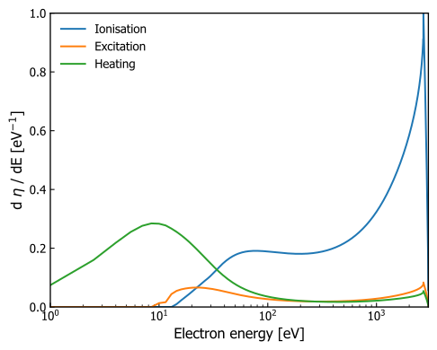
This reproduces Figure 2 of Kozma and Fransson (1992, ApJ, 390, 602–621, doi:10.1086/171296): a pure-oxygen plasma with the electron fraction
x_e = 0.01, with both ionisation and excitation channels. With verbose=True the solver prints its
setup and a per-ion, per-shell breakdown as it runs.
import pynonthermal

n_e = 1e8  # free electron density [cm^-3]
x_e = 1e-2  # ionisation fraction n_OII / (n_OI + n_OII)
n_oxygen = n_e / x_e

# the grid is theirs rather than the default: emin_ev=1 is their low-energy cutoff E_0,
# and emax_ev=3000 is the top of their energy range.
with pynonthermal.SpencerFanoSolver(emin_ev=1, emax_ev=3000, npts=4096, verbose=True) as sf:
    sf.set_temperature(temperature=6000)  # K, for the LTE level populations
    sf.add_element(Z=8, n_elem=n_oxygen, ion_fractions={1: 1 - x_e, 2: x_e}, excitation=True)

    # with fixed ion densities, any positive deposition rate works here: the energy fractions
    # are independent of it (with recomb_ratecoeffs they would not be).
    sf.solve(deposition_ev_per_s_per_cm3=2950.49 * n_oxygen)

    sf.plot_channels(xscalelog=True)
The plot shows the energy distribution of the contributions to ionisation, excitation, and heating. The area under each curve gives the fraction of the deposited energy in that channel:
Units and conventions
- Energies are in eV.
- Number densities are in cm^-3.
- Cross sections are in cm^2.
ion_stage = charge + 1(for example, Fe I hasion_stage=1, Fe II hasion_stage=2).deposition_ev_per_s_per_cm3is in eV s^-1 cm^-3.get_ionisation_ratecoeff()andget_excitation_ratecoeff()both return rates in s^-1.- The
recomb_ratecoeffsofadd_element()are in cm^3 s^-1, keyed by the ion stage that recombines.
Method background
The numerical solver is similar to the Spencer-Fano implementation in the ARTIS radiative transfer code (Shingles et al. (2020, MNRAS, 492, 2029–2043, doi:10.1093/mnras/stz3412)). That code is an independent implementation of Kozma and Fransson (1992, ApJ, 390, 602–621, doi:10.1086/171296), based on the electron slowing-down equation of Spencer and Fano (1954, Phys. Rev., 93, 1172–1181, doi:10.1103/PhysRev.93.1172). CMFGEN uses a similar approach.
The solver discretises the integral form of the Kozma and Fransson degradation equation (their equation 7) on a uniform energy grid as an upper-triangular matrix equation. It solves that equation by back-substitution from the highest energy downward. The SpencerFanoSolver class docstring maps each term of the equation to the method that implements it, and the code comments cite the specific Kozma and Fransson equations at each site. The secondary-electron energy distribution follows Opal, Peterson and Beaty (1971, J. Chem. Phys., 55, 4100–4106, doi:10.1063/1.1676707) as Kozma and Fransson applied it. The energy loss rate to the thermal electrons uses their Coulomb-logarithm prescription, after Schunk and Hays (1971, Planet. Space Sci., 19, 113–117, doi:10.1016/0032-0633(71)90071-7).
The internal level and transition data, which add_ion_excitation() uses, come from the CMFGEN atomic data compilation (see the source data files for references). The solver computes the excitation cross sections from the tabulated collision strengths (Li, Dessart and Hillier 2012, MNRAS, 426, 1671–1686, doi:10.1111/j.1365-2966.2012.21198.x, equation 11). For a permitted transition without a collision strength, it uses the oscillator strength with the approximation of van Regemorter (1962, ApJ, 136, 906–915, doi:10.1086/147445) and the g-bar factor of Mewe (1972, A&A, 20, 215–221), as Shingles et al. (2020, MNRAS, 492, 2029–2043, doi:10.1093/mnras/stz3412) describes in section 2.5.
Cross-section datasets
The ionisation cross sections from H (Z=1) to Ni (Z=28) use the shell-resolved analytical fits of Arnaud and Rothenflug (1985, A&AS, 60, 425–457), with the updates to Fe of Arnaud and Raymond (1992, ApJ, 398, 394–406, doi:10.1086/171864). For the heavier elements (Z>28) and any other ion without a fit, the solver uses the approximation of Axelrod (1980, PhD thesis, University of California, Santa Cruz, equation 3.38). That is the high-energy limit of the formula of Lotz (1967, Z. Phys., 206, 205–211, doi:10.1007/BF01325928) with relativistic corrections, with the subshell binding energies of Lotz (1970, J. Opt. Soc. Am., 60, 206–210, doi:10.1364/JOSA.60.000206).
use_ar1985=True selects the original Arnaud and Rothenflug (1985, A&AS, 60, 425–457) compilation without the Fe updates, for a comparison with older published results.
The Lotz formula has one constant, A in sigma = A q ln(E / P) / (E P). The solver takes it as lotz_a_cm2_ev2 (in cm^2 eV^2). The default of 1.33e-14 is the value of Axelrod (1980). Lotz (1967, Z. Phys., 206, 205–211) gives 4.5e-14 for most shells, available as pynonthermal.axelrod.LOTZ_A_CM2_EV2_LOTZ1967. The fits of Arnaud and Rothenflug (1985) agree with the Lotz value at high energy. The default is therefore a factor of about 3 below both. The solver gives a pynonthermal.LotzApproximationWarning when it adds a Lotz channel, so that the ions that depend on this constant are visible. Filter on that class to silence the warning.
Advanced usage: custom cross sections
Give a cross section as a function of an array of energies in eV that returns cross sections in cm^2
(the type pynonthermal.CrossSectionFunc). The solver calls it on its own grid, and between the grid
points where it needs to, so the plasma does not depend on the energy grid of the solution. The solver
also accepts an array at every energy of sf.engrid. Then the plasma is tied to that grid, and the
solver can only interpolate between the points.
A custom cross section follows the same path through the solver as a built-in one, so the matrix, the energy fractions, and the rate coefficients stay consistent.
import numpy as np
import pynonthermal


def my_ionisation_xs(en_ev):
    return np.interp(en_ev, my_en_ev, my_xs_cm2, left=0.0, right=0.0)


with pynonthermal.SpencerFanoSolver() as sf:
    sf.add_element(Z=8, ion_densities={2: 1.0e8})
    # this keeps the built-in shells and adds one channel; builtin_channels=False replaces them
    sf.add_ionisation_channel(Z=8, ion_stage=2, n_ion=None, ionpot_ev=35.0, xs_vec=my_ionisation_xs, channelkey="mine")
    sf.add_excitation(
        Z=8,
        ion_stage=2,
        levelnumberdensity=None,
        xs_vec=my_excitation_xs,
        epsilon_trans_ev=20.0,
        transitionkey=(0, 3),
        levelpopfrac=0.9,
    )
add_ionisation_channel() takes:
Zandion_stage: the ion that the channel ionises, andn_ion: its number density in cm^-3, orNonefor an ion whose population the solver already holds.ionpot_ev: the ionisation potential in eV, or the excitation energy of the autoionising level of an autoionisation channel. It must lie betweenemin_evandemax_ev. The cross section of a direct-ionisation channel must be zero at and below it. Any value in that range is allowed, so a channel need not be a subshell of the built-in table; a total ionisation cross section for the ion works too.xs_vec: the cross section, non-negative and finite.channelkey: any key that is unique within the ion, for the verbose output.n_ejected,level_energy_ev,auger_electron_energy_ev, andautoionisation: the options of the three sections below, for multiple ionisation, a channel from a metastable level, and excitation autoionisation.
add_excitation() takes:
Z,ion_stage, andlevelnumberdensity: the population of the lower level in cm^-3. GiveNoneinstead, withlevelpopfracbetween 0 and 1, for an ion whose population the solver already holds. The level population then follows the ion population, whether it is fixed or comes from a balance.epsilon_trans_ev: the transition energy in eV. It must be positive and no greater thanemax_ev, since no electron the solver represents could otherwise drive the transition. Transitions belowemin_evare allowed here, butadd_element(excitation=True)drops them. Kozma and Fransson (1992, ApJ, 390, 602–621, doi:10.1086/171296) take every electron belowemin_evto have thermalised, so that energy counts as heating instead.xs_vec, andtransitionkey: the key to pass toget_excitation_ratecoeff().
sf.calculate_N_e() integrates over a domain just above the ionisation potential that is narrower than
one grid cell. A cross section given as a function is called there; an array can only be interpolated, so
resolve that region with npts if it matters for your ion. The term it feeds is the energy that
thermalises below emin_ev, which is a small part of the heating fraction. An
autoionisation channel uses only the values on the grid, as
add_excitation() does.
The solver keeps the Lorentzian secondary-electron distribution of Kozma and Fransson (1992, ApJ, 390, 602–621, doi:10.1086/171296) (their equation 4),
whose width comes from pynonthermal.collion.get_J(). The matrix fill integrates that distribution
analytically, so its shape is not adjustable. An excitation autoionisation
channel does not use that distribution.
Multiple ionisation
A channel of add_ionisation_channel() can remove more than one electron. Set n_ejected to the
number of electrons that one ionisation removes. The ionisation balance of add_element() then sends
the ions of that channel from ion_stage to ion_stage + n_ejected.
The examples below use a made-up cross section with the shape of the Lotz formula. It is zero at and
below its threshold, as a direct-ionisation channel must be. The two examples of the next sections
continue from this one, with the same lotz_like_xs, nist, and recomb.
import numpy as np
import pynonthermal


def lotz_like_xs(threshold_ev, scale_cm2):
    def xs(en_ev):
        u = np.maximum(np.asarray(en_ev, dtype=float) / threshold_ev, 1.0)
        return np.where(u > 1.0, scale_cm2 * np.log(u) / u, 0.0)

    return xs


nist = pynonthermal.collion.get_nist_ionisation_energies_ev()
recomb = {2: 3e-13, 3: 1e-12, 4: 3e-12}
with pynonthermal.SpencerFanoSolver() as sf:
    sf.add_element(Z=38, n_elem=1.0e6, recomb_ratecoeffs=recomb)
    # direct double ionisation of Sr I: the threshold is the sum of the two potentials
    ionpot_ev = nist[(38, 1)] + nist[(38, 2)]
    sf.add_ionisation_channel(
        Z=38,
        ion_stage=1,
        n_ion=None,
        ionpot_ev=ionpot_ev,
        xs_vec=lotz_like_xs(threshold_ev=ionpot_ev, scale_cm2=1e-17),
        channelkey="double",
        n_ejected=2,
    )
    sf.solve(deposition_ev_per_s_per_cm3=1.0)
    print(f"double ionisation rate coefficient {sf.get_ionisation_ratecoeff(Z=38, ion_stage=1, n_ejected=2):.2e} /s")
    print(f"Sr III fraction {sf.get_ion_fractions(Z=38)[3]:.3f}")
The double ionisation sends Sr I ions straight to Sr III, so the Sr III fraction rises above the value without the channel.
Give exclusive channels. Do not include the events of a multiple-ionisation channel in a
single-ionisation cross section of the same ion. If you include them, the solver counts those events
two times. The built-in channels all have n_ejected=1.
The energy of the extra electrons comes from energy conservation, so no Auger data is necessary:
- The primary electron loses
ionpot_evplus the energy of the first ejected electron. The primary electron and the first ejected electron share the energy aboveionpot_ev, as in a single ionisation. The first ejected electron has the Lorentzian distribution (an autoionisation channel is the exception, see below). - By default, the ion keeps the sum of the NIST ground-state potentials from
ion_stagetoion_stage + n_ejected - 1. In general, it keepsionpot_evminusauger_electron_energy_ev. The ionisation fraction counts only the energy that the ion keeps. - The solver treats the
n_ejected - 1extra electrons as Auger electrons. They share the rest of the energy equally, and each appears at that one energy, with the source term of equation 8 of Shingles et al. (2020, MNRAS, 492, 2029–2043, doi:10.1093/mnras/stz3412). An Auger electron at or belowemin_evcounts as heating.
Two cases are typical:
- Inner-shell ionisation followed by Auger decay: set
ionpot_evto the potential of the shell. The extra electrons can then have hundreds of eV. This value ignores fluorescence and excited final states, so it is an upper limit. - Direct multiple ionisation: set
ionpot_evto the sum of the potentials. There is no Auger decay, and the extra electrons appear with zero energy.
The solver compares ionpot_ev with the sum of the potentials, less 1 %
(pynonthermal.collion.MULTIPLE_IONPOT_REL_TOL). Inside that tolerance, the extra electrons get no
energy, and the ion keeps all of ionpot_ev. Below it, the solver gives a UserWarning and does the
same. Give auger_electron_energy_ev to replace the value from energy conservation, for example a
calculated Auger electron energy. If the value leaves the ion less than the sum of the potentials, less
the same 1 %, the solver gives a UserWarning and uses the value. So thresholds from other atomic data,
for example calculated level energies, can differ from NIST. The value is also necessary for an ion that
the NIST data does not have.
Channels from a metastable level
A channel can start from a metastable level of the ion. Give level_energy_ev, the energy of the level
above the ground state. It must be less than the ionisation potential of the ion. The threshold
ionpot_ev is then lower than for the ground state. For a multiple ionisation or an autoionisation, the
ion must keep the sum of the NIST potentials less level_energy_ev, and the default
auger_electron_energy_ev increases by level_energy_ev. A single direct ionisation has no such check.
n_ion stays the population of the whole ion, as for every channel. The channel rate uses that
population. Scale the cross section by the population fraction of the level.
level_energy_ev = 1.8  # a metastable level of Sr I, 1.8 eV above the ground state
level_popfrac = 0.2  # the fraction of the Sr I ions in that level
with pynonthermal.SpencerFanoSolver() as sf:
    sf.add_element(Z=38, n_elem=1.0e6, recomb_ratecoeffs=recomb)
    # double ionisation from the level: the threshold is the ground-state sum less the level energy
    ionpot_ev = nist[(38, 1)] + nist[(38, 2)] - level_energy_ev
    double_xs = lotz_like_xs(threshold_ev=ionpot_ev, scale_cm2=1e-17)
    sf.add_ionisation_channel(
        Z=38,
        ion_stage=1,
        n_ion=None,
        ionpot_ev=ionpot_ev,
        xs_vec=lambda en_ev: level_popfrac * double_xs(en_ev=en_ev),
        channelkey="double_meta",
        n_ejected=2,
        level_energy_ev=level_energy_ev,
    )
    sf.solve(deposition_ev_per_s_per_cm3=1.0)
    print(f"double ionisation rate coefficient {sf.get_ionisation_ratecoeff(Z=38, ion_stage=1, n_ejected=2):.2e} /s")
Without level_energy_ev, the same call gives a UserWarning, because the threshold is below the sum
of the ground-state potentials, and the Auger electron gets zero energy.
Excitation autoionisation
An excitation autoionisation is an excitation to a level above the ionisation limit, which then
autoionises. Such a channel does not give the Lorentzian distribution of secondary electrons. The primary
electron loses exactly the excitation energy, as in add_excitation(), and the ion emits an Auger
electron of one energy. Set autoionisation=True. Set ionpot_ev to the excitation energy of the
autoionising level. The solver sets the cross section below that energy to zero, as
add_excitation() does, and it keeps the value at that energy.
with pynonthermal.SpencerFanoSolver() as sf:
    sf.add_element(Z=38, n_elem=1.0e6, recomb_ratecoeffs=recomb)
    # an autoionising level of Sr I at 20 eV, which is 14.3 eV above the ionisation limit. The
    # Auger electron gets those 14.3 eV, and the ion keeps the 5.7 eV ionisation potential.
    sf.add_ionisation_channel(
        Z=38,
        ion_stage=1,
        n_ion=None,
        ionpot_ev=20.0,
        xs_vec=lotz_like_xs(threshold_ev=20.0, scale_cm2=1e-16),
        channelkey="eai",
        autoionisation=True,
    )
    sf.solve(deposition_ev_per_s_per_cm3=1.0)
    print(
        f"Sr I ionisation rate coefficient {sf.get_ionisation_ratecoeff(Z=38, ion_stage=1):.2e} /s (built-in shells + eai)"
    )
    print(f"Sr I ionisation fraction {sf.get_frac_ionisation_ion(Z=38, ion_stage=1):.4f}")
The same cross section as a direct channel (autoionisation=False) would count all 20 eV as ionisation
energy and would give the ejected electron the Lorentzian distribution. With autoionisation=True, the
ionisation fraction of Sr I is lower, and the heating fraction is higher.
The energy rules follow those of a multiple ionisation:
- All
n_ejectedelectrons appear at the energyauger_electron_energy_ev / n_ejected, with the source term of the Auger electrons in equation 8 of Shingles et al. (2020, MNRAS, 492, 2029–2043, doi:10.1093/mnras/stz3412). By default,auger_electron_energy_evisionpot_evpluslevel_energy_evminus the sum of the NIST potentials fromion_stagetoion_stage + n_ejected - 1. That is the energy of the level above the ionisation limit. Give a value to replace the default. An electron at or belowemin_evcounts as heating. - The ion keeps
ionpot_evminusauger_electron_energy_ev, and the ionisation fraction counts only that energy. - The rate coefficient and the ionisation balance count the channel as an ionisation of
n_ejectedelectrons.get_ionisation_ratecoeff()includes it in the total of the ion.
Give an exclusive cross section. Do not include the events of an autoionisation channel in a direct-ionisation channel of the same ion. Many autoionising levels can share one channel with the sum of their cross sections, or a few channels with binned excitation energies. The excitation energy of a shared channel must be the lowest one of its levels, because the cross section must be zero below it. The default Auger electron energy then comes from that lowest level.
Citing pynonthermal
If you use pynonthermal, please cite it through the Zenodo record. Please also consider a citation of the papers that describe the method: Kozma and Fransson (1992, ApJ, 390, 602–621, doi:10.1086/171296) and Shingles et al. (2020, MNRAS, 492, 2029–2043, doi:10.1093/mnras/stz3412).
License
Distributed under the MIT license. See LICENSE for details.
1 maintainer

Metadata
1 maintainer
Release files for pynonthermal 2026.9.30
For a detailed explanation of source distributions (sdists) and built distributions (wheels), please see the package formats documentation.
Source distribution (sdist)
| File | Size | Uploaded | |
|---|---|---|---|
| pynonthermal-2026.9.30.tar.gz | 5.8 MB | Details |
Built distribution (wheel)
| File | Interpreter | ABI | Platform | Reset |
|---|---|---|---|---|
| pynonthermal-2026.9.30-py3-none-any.whl | Python 3 | none | any | Details |
Total release size: 11.4 MB
Release files / pynonthermal-2026.9.30.tar.gz
| Download URL | pynonthermal-2026.9.30.tar.gz |
|---|---|
| Size | 5.8 MB |
| Tags | Source |
|
SHA-256 checksum How to use checksums |
38019bc5f5e5f4b196b2c5e762171c6d202c3f379fb73694d0a472040ad1a587
|
|
BLAKE2b-256 checksum How to use checksums |
51f9604fd63345b49522c35c0c2e99aad116e8b2fff581961bdebbf41d7adb96
|
| Upload date | |
|
Uploaded using Trusted Publishing? What is trusted publishing? |
Yes |
| Uploaded via |
twine/7.0.0 CPython/3.13.14
|
Provenance
Provenance describes where a file came from. On PyPI, provenance is shared via attestations, which provide a verifiable record of the build or publishing details. View details, limitations and caveats.


PyPI Publish Attestation
PyPI verified that this artifact, at this checksum, originated from the publisher listed below.
Signed by GitHub Actions, verified by PyPI on Sep 30, 2026.
Transparency logRelease files / pynonthermal-2026.9.30-py3-none-any.whl
| Download URL | pynonthermal-2026.9.30-py3-none-any.whl |
|---|---|
| Size | 5.6 MB |
| Tags | Python 3 |
|
SHA-256 checksum How to use checksums |
a169621a5dc4b5fda09e20b84052229052b3839e6582fd2d797e7e1d5d8a0382
|
|
BLAKE2b-256 checksum How to use checksums |
037280129d99132d4aa4ee58ae29f9623fa38c1f10e338fa066a2c7c34c88d15
|
| Upload date | |
|
Uploaded using Trusted Publishing? What is trusted publishing? |
Yes |
| Uploaded via |
twine/7.0.0 CPython/3.13.14
|
Provenance
Provenance describes where a file came from. On PyPI, provenance is shared via attestations, which provide a verifiable record of the build or publishing details. View details, limitations and caveats.
PyPI Publish Attestation
PyPI verified that this artifact, at this checksum, originated from the publisher listed below.
Signed by GitHub Actions, verified by PyPI on Sep 30, 2026.
Transparency log













