PyOKNN 0.1.66

A spatial lag operator proposal implemented in Python21: only the k-nearest neighbor (oknn), PyOKNN.

PyOKNN - A spatial lag operator proposal implemented in Python: only the k-nearest neighbor (oknn).

Why

By opposition to the time-series case, specifying the spatial lag operator involves a lot of arbitrariness. Hence this proposal, which yields a lag operator usable as primarily observed without modifications. (click to expand)

Fingleton (2009) and Corrado and Fingleton (2012) remind the analogies between temporal and spatial processes, at least when considering their lag operators. In the spatial econometric (SE) case, the lag operator is always explicitly involved via the use of a matrix , where is the number of interacting positions. The chosen space can be geographic, economic, social or of any other type. In the temporal case, which is seen as a space like no other given its inescapable anisotropic nature, the lag operator is in practice never explicitly considered. Any variable to lag, say, a vector , is formed over components that are prealably sorted according to their position on the timeline. This allows the lag-procedure to simply consist of offsetting down/up these components by a lag-determined number of rows, say, one row. In matrix terms, this offsetting procedure would be entirely equivalent to pre-multiplying an unsorted version of by a boolean matrix with s indicating the immediate and unilateral proximity between temporal positions.

The so-structured data generating process (DGP) thus involves as primarily observed, i.e. with no restructuring hypothesis or transformation. For each lag, this provides the statistician with a straightforward parameter space definition, whose knowledge of the exact boundary is important, both for estimation and inference (Elhorst et al., 2012).

By opposition to the time series (TS) case, specifying involves a lot of arbitrariness. Apart from ’s non-nilpotency, these hypotheses deal with ’s isotropy (Cressie, 1993) and finding ’s true entrywise specification through a very large number of competing ones, be it functional or binary. Some famous entrywise specifications are the negative exponential function (Haggett, 1965), the inverse-distance function (Wilson, 1970), the combined distance-boundary function (Cliff and Ord, 1973) and the weighted logistic accessibility function (Bodson and Peeters, 1975). Binary weights specifications are either based on the k-nearest neighbor (knn), on the k-order of contiguity or on the radial distance. Then, to ensure the unique definition of any to-be-lagged variable in terms of the other variables of the model, is scaled depending on the choice one makes among three competing normalization techniques. The first one makes row-stochastic, but does not necessarily preserve its symmetry. The second one pre- and post-multiplies by the negative square root of a diagonal matrix reporting its row-totals (Cliff and Ord, 1973). The last one scales by its largest characteristic root (Elhorst, 2001).

But the choice of and of its transformation is not innocuous. For a maximum likelihood (ML) estimation to be consistent, the estimated spatial model must involve the true (Dogan, 2013; Lee, 2004). When dealing with autoregressive disturbances, both estimators ML and spatial generalized moments (GM) (Anselin, 2011; Arraiz et al., 2010; Drukker et al., 2013; Kelejian and Prucha, 2010) theoretically base their knowledge of unobservable innovations upon the knowledge of . When facing endogeneity problems in non-autoregressive specifications and resorting to, e.g. Kelejian and Prucha (1999)’s generalized moments estimator (GM), the definition of the exogeneity constrains heavily relies on , which yields consistent and efficient estimations for sure, but potentially not with respect to the true DGP. If resorting to the instrumental variables (IV) method – in which space is conceived as providing ideal instruments (Das et al., 2003; Lee, 2003; Pinkse and Slade, 2010) –, the strength of instruments is far from being ensured with in its most common specification, i.e. whose lag consists of neighbors-averaging. Moreover, as discussed by Gibbons and Overman (2012), the inclusion of the product of higher powers of the spatial lag operator in the set of instruments is very likely to lead to a problem of colinearity, which in turn leads to the weaknesses of both identification and instruments. Finally, when computing LeSage and Pace (2009)’s total direct and indirect effects, the correctness of the true derivative of the regressand with respect to any spatially filtered variable is a direct result of the correctness of .

Hence the proposal that follows, i.e a specification method for the spatial lag operator whose properties are as close as possible to the ones of its time series (TS) counterpart, i.e. usable as primarily observed without modifications. Nonetheless we follow Pinkse and Slade (2010, p.105)’s recommendation of developing tools that are not simply extensions of familiar TS techniques to multiple dimensions. This is done so by proposing a specification-method which is fully grounded on the observation of the empirical characteristics of space, while minimizing as much as possible the set of hypotheses that are required.

Whereas the oknn specification of is the strict spatial counterpart of the k-order TS lag operator, , it had surprisingly never been proposed. The likely reason for this fact is the usual assumption of regular lattice, on which the autoregression structure superimposes. Frequently seen as an issue, the irregularity of the lattice is the rational for this specification. Moreover, in realistic spatial configurations, the lattice regularity is the exception rather than the rule.

This specification implies the transposition in space of the three-stage modeling approach of Box and Jenkins (1976) which consists of (i) identifying and selecting the model, (ii) estimating the parameters and (iii) checking the model. It follows that the models that are subject to selection in the present work are likely to involve a large number of parameters whose distributions, probably not symmetrical, are cumbersome to derive analytically. This is why in addition to the (normal-approximation-based) observed confidence intervals, (non-adjusted and adjusted) bootstrap percentile intervals are implemented. However, the existence of fixed spatial weight matrices prohibits the use of traditional bootstrapping methods. So as to compute (normal approximation or percentile-based) confidence intervals for all the parameters, we use a special case of bootstrap method, namely Lin et al. (2007)’s hybrid version of residual-based recursive wild bootstrap. This method is particularly appropriate since it (i) "accounts for fixed spatial structure and heteroscedasticity of unknown form in the data" and (ii) "can be used for model identification (pre-test) and diagnostic checking (post-test) of a spatial econometric model". As mentioned above, non-adjusted percentile intervals as well as bias-corrected and accelerated (BCa) percentile intervals (Efron and Tibshirani, 1993) are implemented as well.

How

Python2.7.+ requirements

• matplotlib (==1.4.3 preferably)
• numdifftools (>=0.9.20 preferably)
• numpy (>=1.14.0 preferably)
• pandas (>=0.22.0 preferably)
• scipy (>=1.0.0 preferably)
• pysal (>=1.14.3 preferably)

Installation

We are going to use a package management system to install and manage software packages written in Python, namely pip. Open a session in your OS shell prompt and type

pip install pyoknn

Or using a non-python-builtin approach, namely git,

git clone git://github.com/lfaucheux/PyOKNN.git
cd PyOKNN
python setup.py install

Example usage:

The example that follows is done via the Python Shell. Let's first import the module PyOKNN.

>>> import PyOKNN as ok  

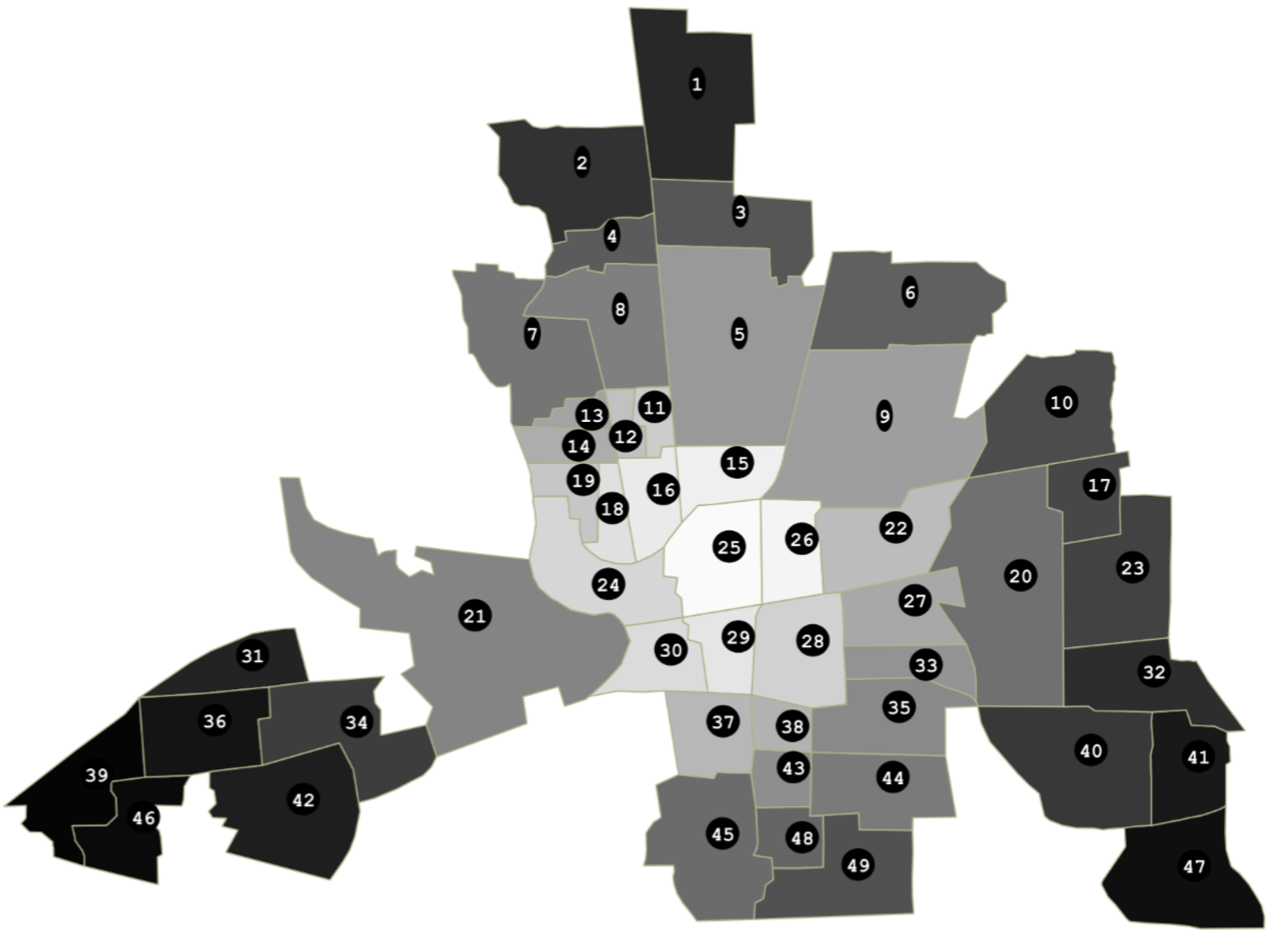
We use Anselin's Columbus OH 49 observation data set. Since the data set is included in PyOKNN, there is no need to mention the path directory.

>>> o = ok.Presenter(
...     data_name = 'columbus',
...     y_name    = 'CRIME',
...     x_names   = ['INC', 'HOVAL'],
...     id_name   = 'POLYID',
...     verbose   = True,
...     opverbose = True,
... )

Let's directly illustrate the main raison d'être of this package, i.e. modelling spatial correlation structures. To do so, simply type

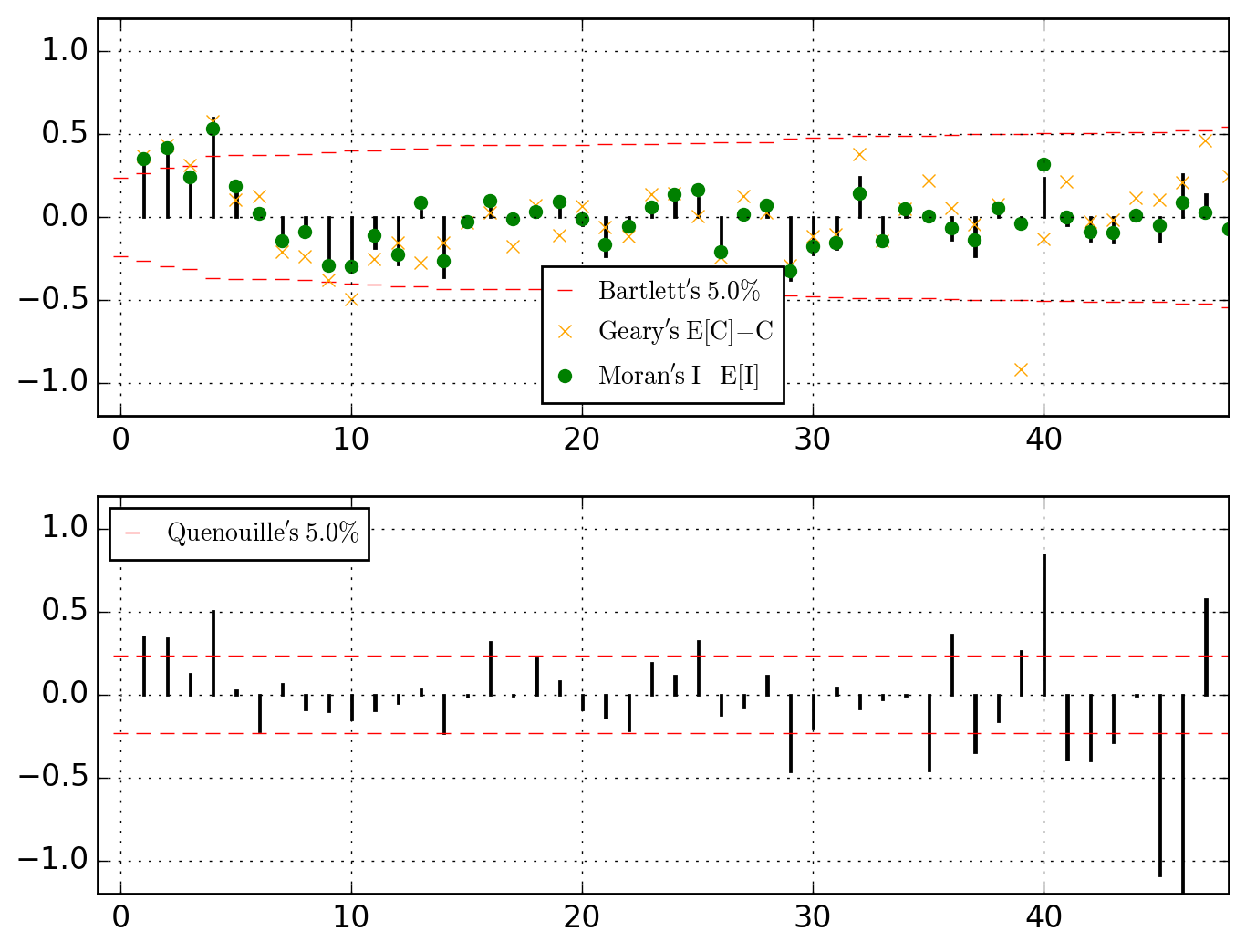
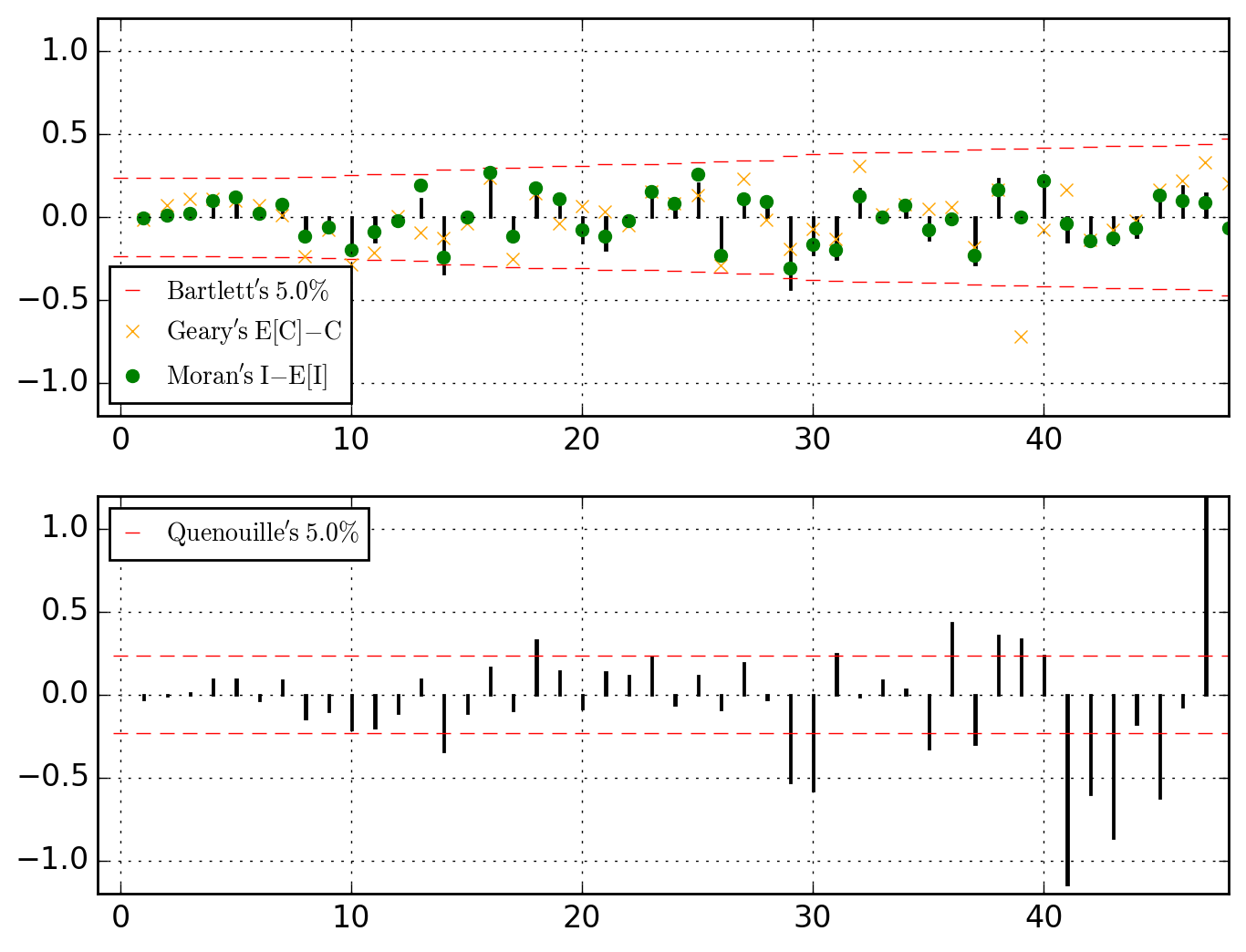
>>> o.u_XACF_chart
saved in  C:\data\Columbus.out\ER{0}AR{0}MA{0}[RESID][(P)ACF].png

and

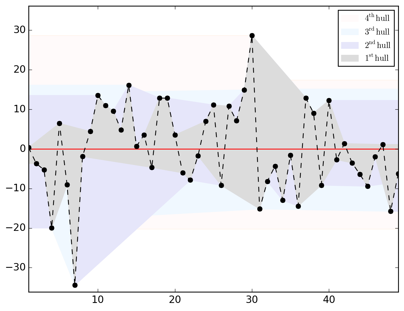
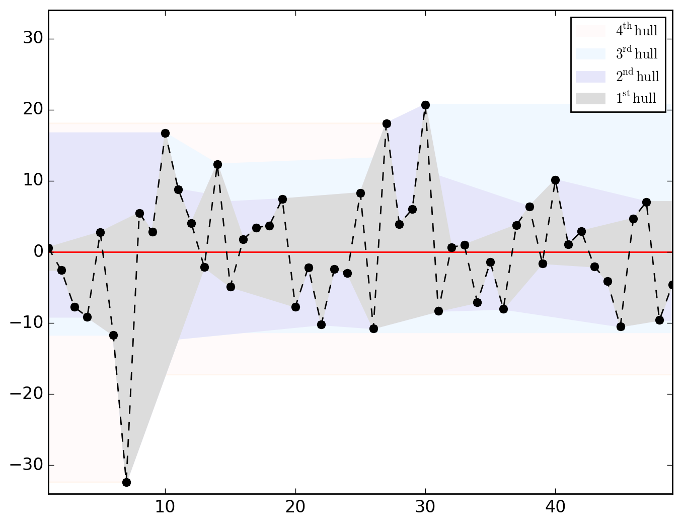
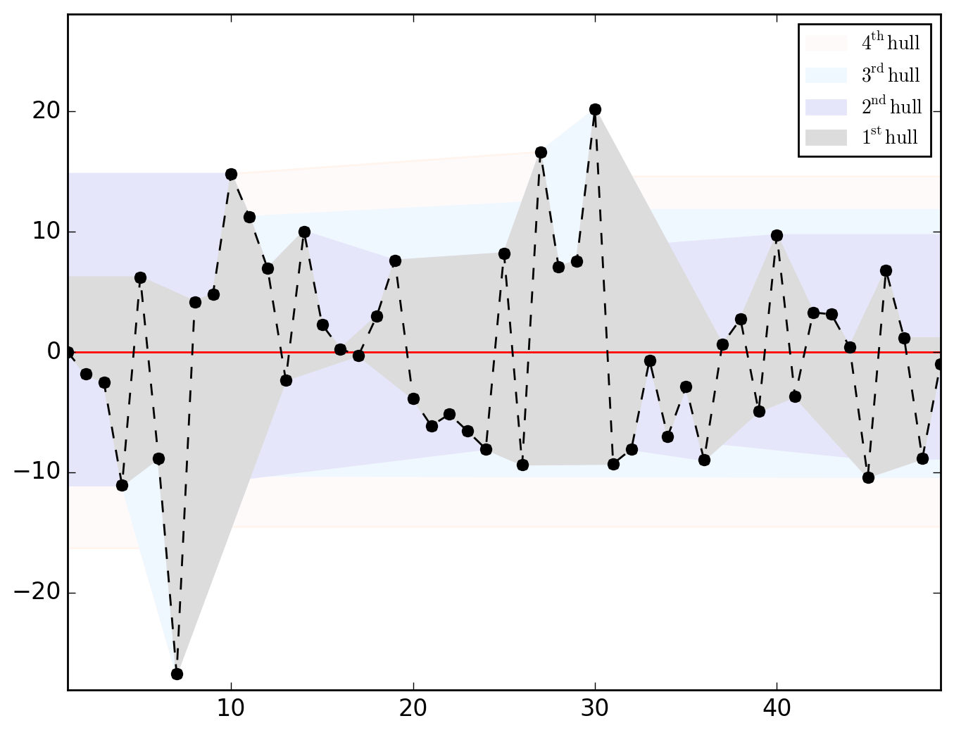
>>> o.u_hull_chart
saved in  C:\data\Columbus.out\ER{0}AR{0}MA{0}[RESID][HULLS].png

ER{0}AR{0}MA{0}[RESID][(P)ACF].png and ER{0}AR{0}MA{0}[RESID][HULLS].png look like this

N.B.. (click to expand)

Hull charts should be treated with great caution since before talking about "long-distance trend" and/or "space-dependent variance", we should make sure that residuals are somehow sorted geographically. However, as shown in the map below, saying that it is totally uninformative appears abusive.

Be it in the ACF (upper dial) or in the PACF, we clearly have significant dependences at work through the lags 1, 2 and 4. Let's first think of it as global (thus considering the PACF) and go for an AR{1,2,4}.

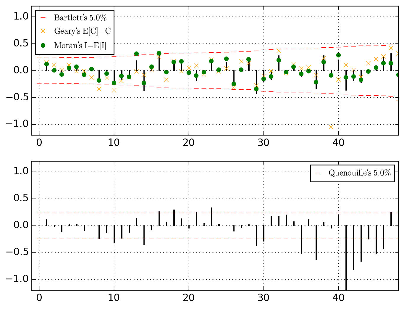
>>> o.u_XACF_chart_of(AR_ks=[1, 2, 4])
Optimization terminated successfully.
         Current function value: 108.789436
         Iterations: 177
         Function evaluations: 370
saved in  C:\data\Columbus.out\ER{0}AR{1,2,4}MA{0}[RESID][(P)ACF].png
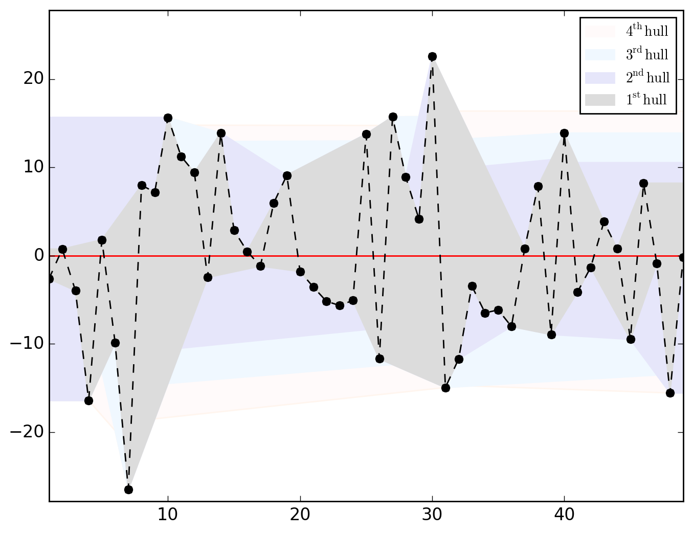
>>> o.u_hull_chart
saved in  C:\data\Columbus.out\ER{0}AR{1,2,4}MA{0}[RESID][HULLS].png

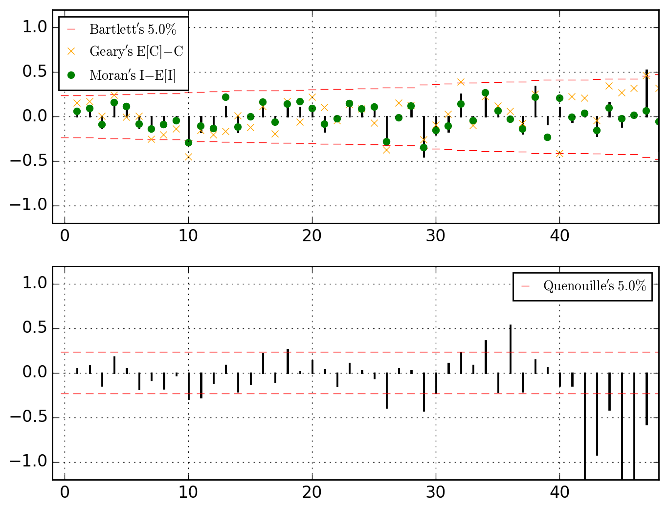
or thinking of those as local, let's go for a MA{1,2,4}.

>>> o.u_XACF_chart_of(MA_ks=[1, 2, 4])
Optimization terminated successfully.
         Current function value: 107.015463
         Iterations: 174
         Function evaluations: 357
saved in  C:\data\Columbus.out\ER{0}AR{0}MA{1,2,4}[RESID][(P)ACF].png
>>> o.u_hull_chart
saved in  C:\data\Columbus.out\ER{0}AR{0}MA{1,2,4}[RESID][HULLS].png

Thinking of CRIME variable as cointegrated through space with INC and HOVAL, let's run a (partial) differencing whose structure is superimposed to the lags 1, 2 and 4.

>>> o.u_XACF_chart_of(ER_ks=[1, 2, 4])             
Optimization terminated successfully.
         Current function value: 107.126738
         Iterations: 189
         Function evaluations: 382
saved in  C:\data\Columbus.out\ER{1,2,4}AR{0}MA{0}[RESID][(P)ACF].png
>>> o.u_hull_chart
saved in  C:\data\Columbus.out\ER{1,2,4}AR{0}MA{0}[RESID][HULLS].png

A little summary is always useful.

>>> o.summary()
================================= PARS
\\\\ HAT ////  ER{0}AR{0}MA{0}  ER{0}AR{0}MA{1,2,4}  ER{0}AR{1,2,4}MA{0}  ER{1,2,4}AR{0}MA{0}
\beta_0              68.618961            63.418312            40.602532            59.163974
\beta_{HOVAL}        -0.273931            -0.290030            -0.261453            -0.251289
\beta_{INC}          -1.597311            -1.237462            -0.936830            -1.147231
\gamma_{1}                 NaN                  NaN                  NaN             0.106979
\gamma_{2}                 NaN                  NaN                  NaN             0.212151
\gamma_{4}                 NaN                  NaN                  NaN             0.377095
\lambda_{1}                NaN             0.233173                  NaN                  NaN
\lambda_{2}                NaN             0.303743                  NaN                  NaN
\lambda_{4}                NaN             0.390871                  NaN                  NaN
\rho_{1}                   NaN                  NaN             0.137684                  NaN
\rho_{2}                   NaN                  NaN             0.218272                  NaN
\rho_{4}                   NaN                  NaN             0.144365                  NaN
\sigma^2_{ML}       122.752913            93.134974            79.000511            69.257032
================================= CRTS
\\\\ HAT ////         ER{0}AR{0}MA{0}  ER{0}AR{0}MA{1,2,4}  ER{0}AR{1,2,4}MA{0}  ER{1,2,4}AR{0}MA{0}
llik                      -187.377239          -176.543452          -178.317424          -176.654726
HQC                        382.907740           369.393427           372.941372           369.615976
BIC                        386.429939           376.437825           379.985770           376.660374
AIC                        380.754478           365.086903           368.634848           365.309452
AICg                         5.625770             5.306023             5.378430             5.310565
pr^2                         0.552404             0.548456             0.542484             0.550022
pr^2 (pred)                  0.552404             0.548456             0.590133             0.550022
Sh's W                       0.977076             0.990134             0.949463             0.972979
Sh's Pr(>|W|)                0.449724             0.952490             0.035132             0.316830
Sh's W (pred)                0.977076             0.978415             0.969177             0.973051
Sh's Pr(>|W|) (pred)         0.449724             0.500748             0.224519             0.318861
BP's B                       7.900442             2.778268            20.419370             9.983489
BP's Pr(>|B|)                0.019250             0.249291             0.000037             0.006794
KB's K                       5.694088             2.723948             9.514668             6.721746
KB's Pr(>|K|)                0.058016             0.256155             0.008588             0.034705 

Given that the specification ER{0}AR{0}MA{1,2,4} has the minimum BIC, let's pursue with it and check its parameters-covariance matrix and statistical table. Keep in mind that the returned statistics and results are always those of the last model we worked with. We can figure out what this last model is -- i.e. the ongoing model --, typing

>>> o.model_id
ER{1,2,4}AR{0}MA{0}

Since we want to continue with the specification ER{0}AR{0}MA{1,2,4}, we thus have to explicitly set it as "ongoing". This can be done, say, while requesting the parameters-covariance matrix and statistical table, as follows

>>> o.covmat_of(MA_ks=[1, 2, 4])
\\\\ COV ////    \beta_0  \beta_{INC}  \beta_{HOVAL}  \lambda_{1}  \lambda_{2}  \lambda_{4}  \sigma^2_{ML}
\beta_0        19.139222    -0.784264      -0.025163    -0.061544    -0.028639     0.073201      -1.621429
\beta_{INC}    -0.784264     0.109572      -0.019676     0.008862     0.017765    -0.014063       0.715907
\beta_{HOVAL}  -0.025163    -0.019676       0.007814    -0.001673    -0.006111     0.003102      -0.239979
\lambda_{1}    -0.061544     0.008862      -0.001673     0.010061    -0.000185    -0.001523       0.346635
\lambda_{2}    -0.028639     0.017765      -0.006111    -0.000185     0.014815    -0.001668       0.576185
\lambda_{4}     0.073201    -0.014063       0.003102    -0.001523    -0.001668     0.008075       0.092086
\sigma^2_{ML}  -1.621429     0.715907      -0.239979     0.346635     0.576185     0.092086     394.737828

and

>>> o.table_test # no need to type `o.table_test_of(MA_ks=[1, 2, 4])`
\\\\ STT ////   Estimate  Std. Error  t|z value      Pr(>|t|)      Pr(>|z|)  95.0% lo.  95.0% up.
\beta_0        63.418312    4.374840  14.496146  3.702829e-18  1.281465e-47  62.193379  64.643245
\beta_{INC}    -1.237462    0.331017  -3.738367  5.422541e-04  1.852193e-04  -1.330145  -1.144779
\beta_{HOVAL}  -0.290030    0.088398  -3.280974  2.056930e-03  1.034494e-03  -0.314781  -0.265279
\lambda_{1}     0.233173    0.100303   2.324690  2.487823e-02  2.008854e-02   0.205089   0.261257
\lambda_{2}     0.303743    0.121716   2.495501  1.649425e-02  1.257793e-02   0.269663   0.337823
\lambda_{4}     0.390871    0.089860   4.349759  8.232171e-05  1.362874e-05   0.365711   0.416032
\sigma^2_{ML}  93.134973   19.868010   4.687685  2.795560e-05  2.763129e-06  87.572032  98.697913

Incidentally, note that the above table holds for

>>> o.type_I_err
0.05

But one may want not to make any assumptions regarding spatial parameters distribution and favor an empirical approach by bootstrap-estimating all parameters as well as their (bias-corrected and accelerated - BCa) percentile intervals.

>>> o.opverbose = False       # Printing minimizer's messages may slow down iterations
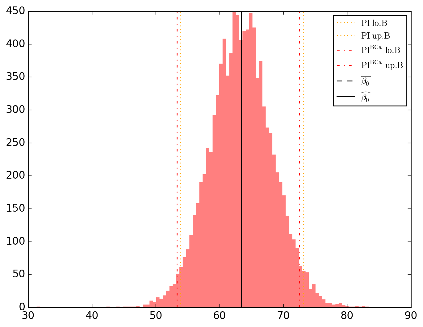
>>> o.PIs_computer(
...     plot_hist = True,     # Bootstrap distributions
...     plot_conv = True,     # Convergence plots
...     MA_ks     = [1, 2, 4]
...     nbsamples = 10000     # Number of resamplings
... )

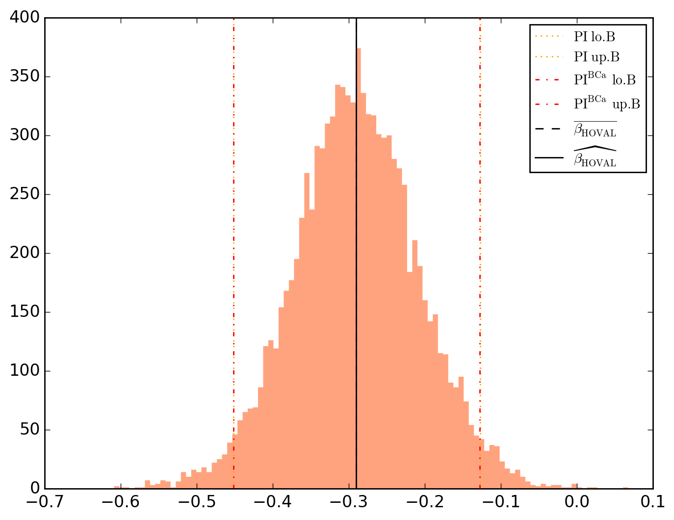
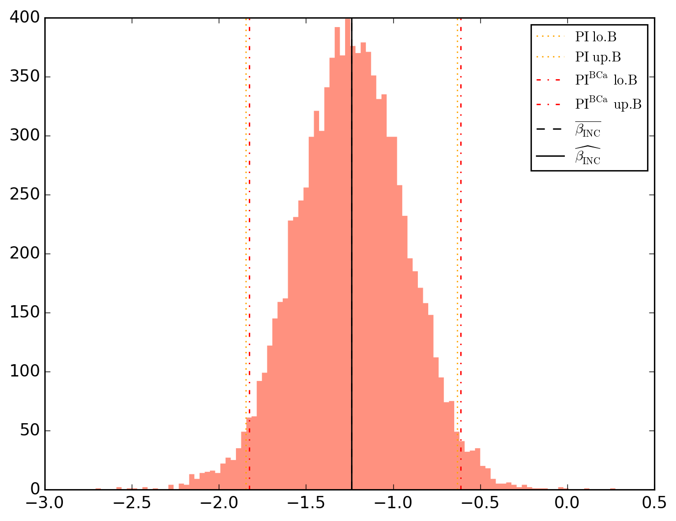
10000 resamplings later, we see regarding economic parameters that using normal-approximation-based confidence intervals is anything but "flat wrong", look:

which is not as true for spatial parameters:

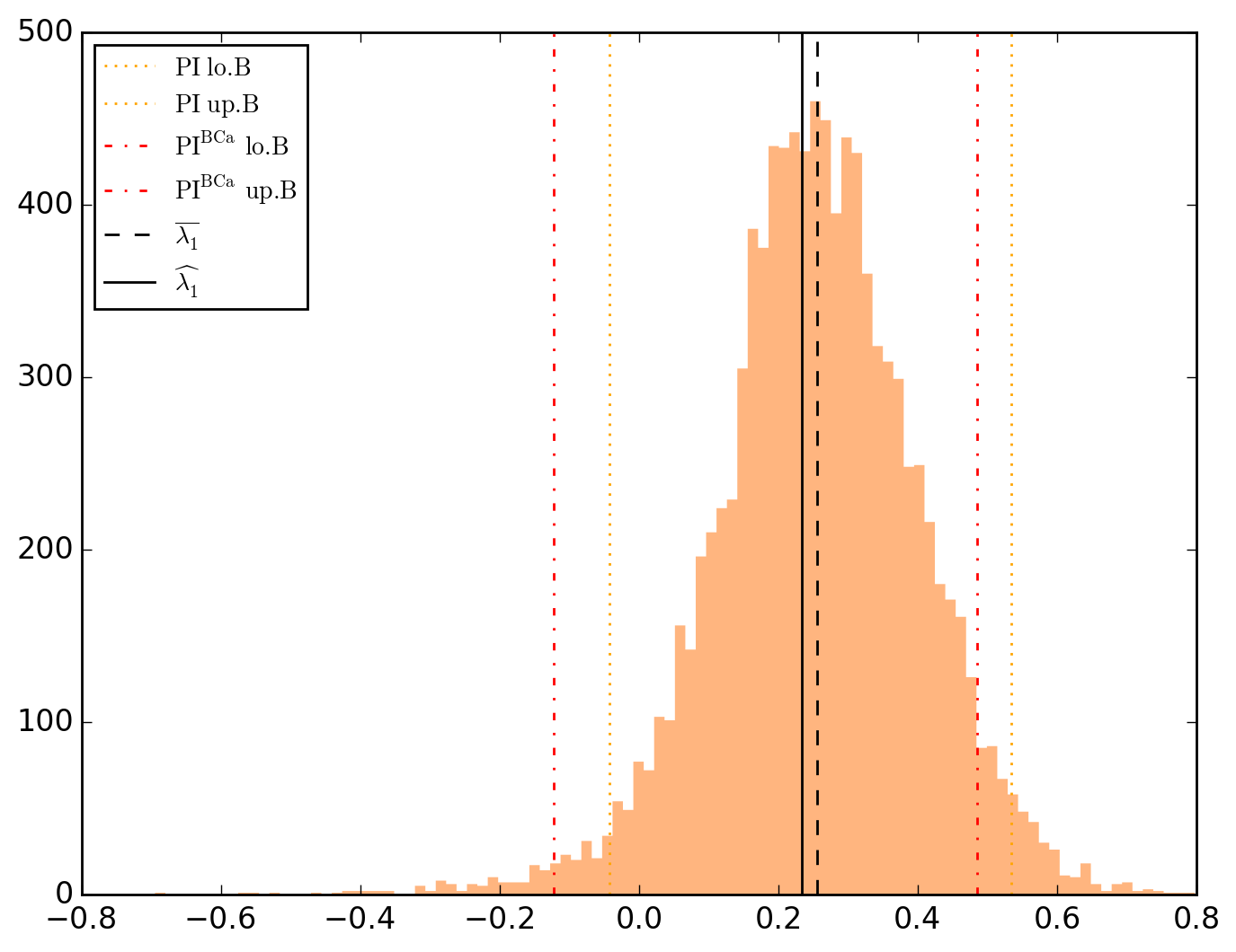
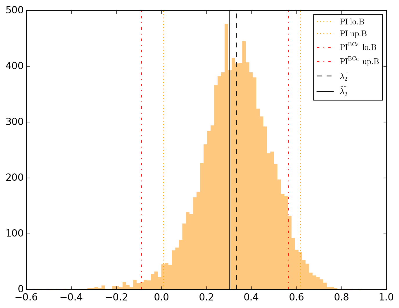
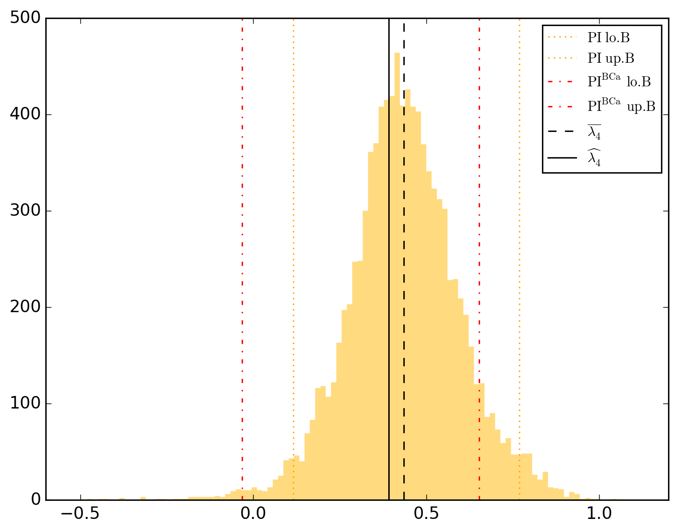
One notable diffference is that BCa percentile intervals of and contain 0 while their non-BCa version does not. Moreover, these non-normal-based intervals are all the more informative when dealing with asymmetrical distributions, as that of

Note that the statistical table, previously called typing o.table_test, is now augmented on the right by the bootstrap-results.

>>> o.table_test
\\\\ STT ////   Estimate  Std. Error  t|z value      Pr(>|t|)      Pr(>|z|)  95.0% CI.lo.  95.0% CI.up.  95.0% PI.lo.  95.0% PI.up.  95.0% BCa.lo.  95.0% BCa.up.
\beta_0        63.418312    4.374840  14.496146  3.702829e-18  1.281465e-47     62.193379     64.643245     53.922008     73.107011      53.328684      72.512817
\beta_{INC}    -1.237462    0.331017  -3.738367  5.422541e-04  1.852193e-04     -1.330145     -1.144779     -1.846416     -0.632656      -1.825207      -0.610851
\beta_{HOVAL}  -0.290030    0.088398  -3.280974  2.056930e-03  1.034494e-03     -0.314781     -0.265279     -0.451431     -0.127206      -0.451658      -0.127696
\lambda_{1}     0.233173    0.100303   2.324690  2.487823e-02  2.008854e-02      0.205089      0.261257     -0.043012      0.534407      -0.122474       0.484635
\lambda_{2}     0.303743    0.121716   2.495501  1.649425e-02  1.257793e-02      0.269663      0.337823      0.008517      0.616936      -0.089690       0.562511
\lambda_{4}     0.390871    0.089860   4.349759  8.232171e-05  1.362874e-05      0.365711      0.416032      0.116317      0.768369      -0.032977       0.652651
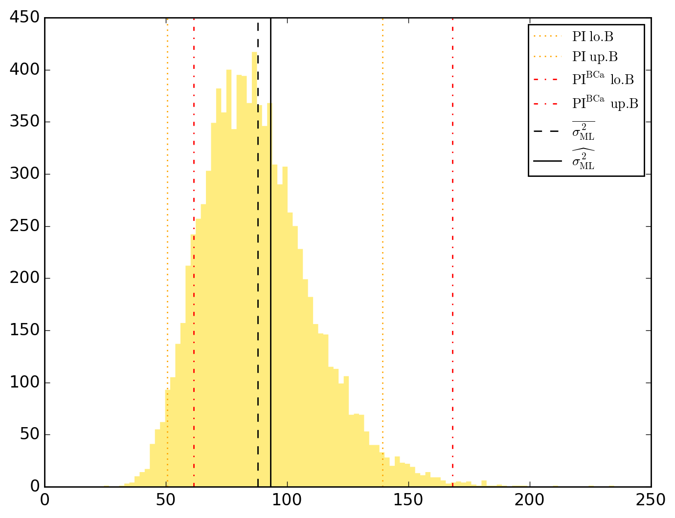
\sigma^2_{ML}  93.134973   19.868010   4.687685  2.795560e-05  2.763129e-06     87.572032     98.697913     50.668029    139.392307      61.426042     168.070074

Incidentally, other distributions have been generated in addition to those of the parameters

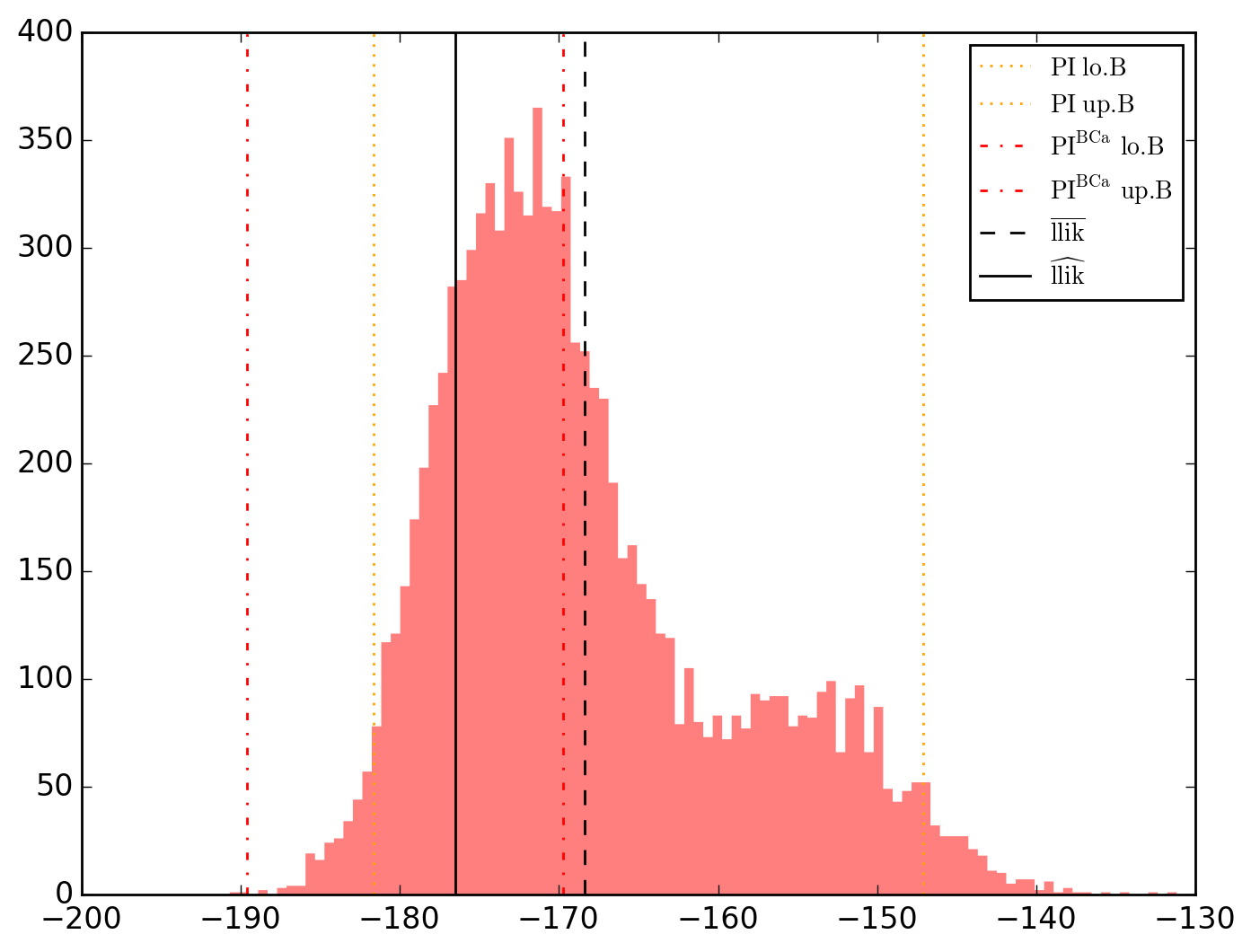
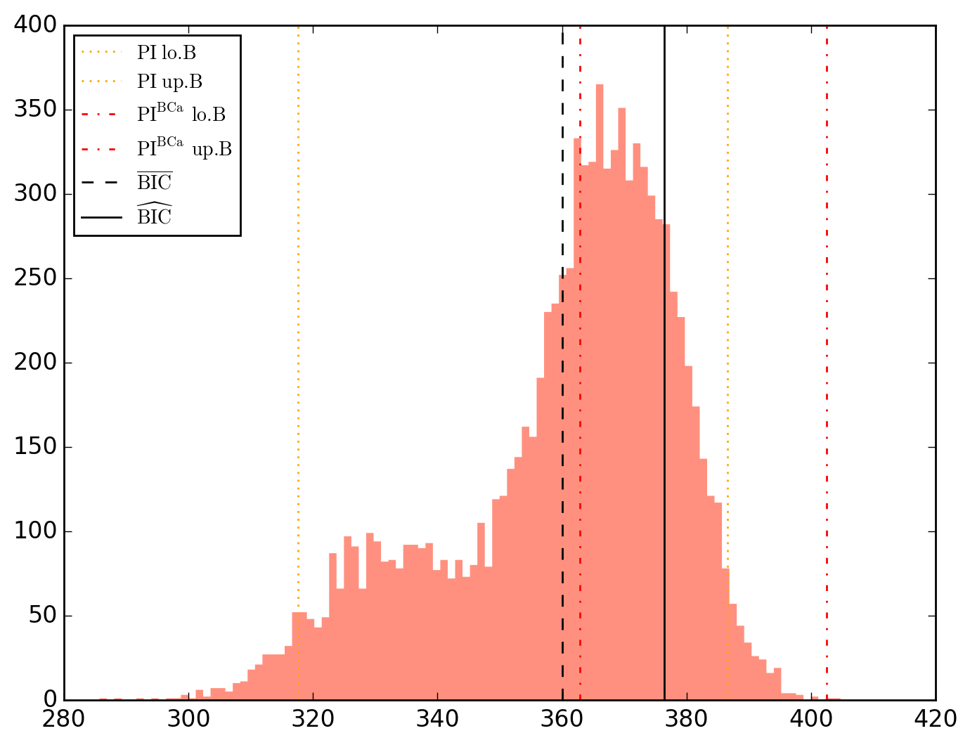
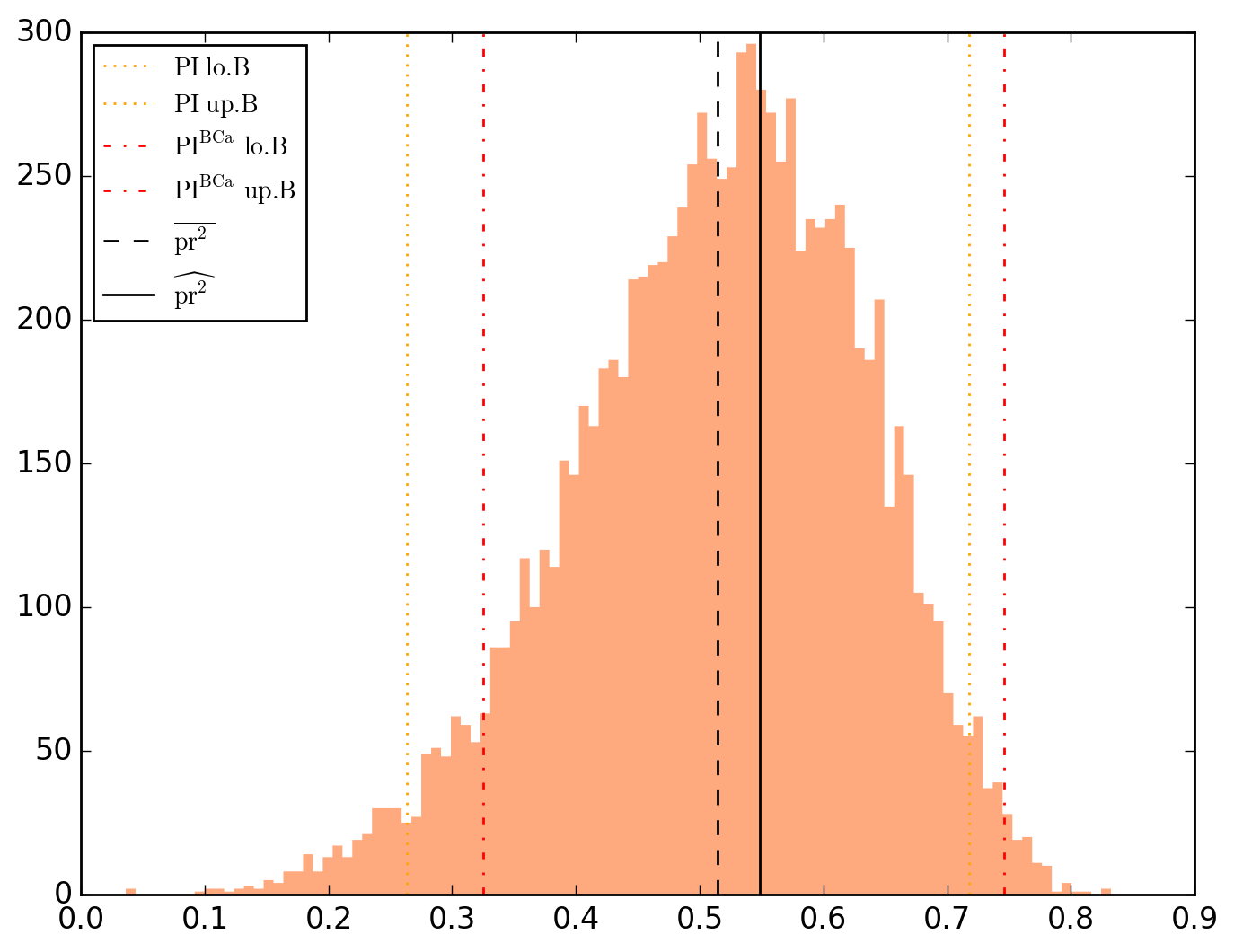
All the other charts (distributions and convergence plots) are viewable here.