A python library for simulating and analyzing microscope point spread functions (PSFs)

Project description


pyotf
A simulation software package for modelling optical transfer functions (OTF)/point spread functions (PSF) of optical microscopes written in python.
Introduction
The majority of this package's documentation is included in the source code and should be available in any interactive session. The intent of this document is to give a quick overview of the package's features and potential uses. Much of the code has been designed with interactive sessions in mind but it should still be usable in larger scripts and programs.
Installation
Installation is simplest with conda or pip:
conda install -c david-hoffman pyotf
pip install pyotf
Components
The package is made up of four component modules:
otf.pywhich contains classes for generating different types of OTFs and PSFsphase_retrieval.pywhich contains functions and classes to perform iterative phase retrieval of the rear aperature of the optical systemzernike.pywhich contains functions for calculating Zernike Polynomialsutils.pywhich contains various utility functions used throughout the package.
otf.py
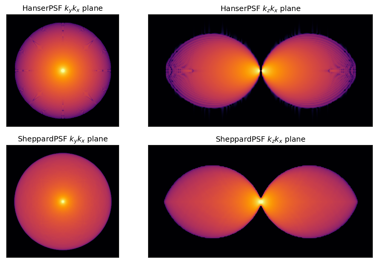
Two models of optical imaging systems are available in this module one described by Hanser et al and one described by Arnison and Sheppard. They are, in fact, mathematically equivalent but in practice each have their strengths and weaknesses. A big benefit of HanserPSF is that it allows one to calculate selected z planes of the PSF. However, if the choosen z-planes are not equispaced then the field OTF (OTFa) and intensity OTF (OTFi) calculated from the model won't make physical sense.
Both the SheppardPSF and HanserPSF have much the same interface. When instantiating them the user must provide a set of model parameters. To fully describe a PSF or OTF of an objective lens, assuming no abberation, we generally need a few parameters:
- The wavelength of operation (assume monochromatic light)
- the numerical aperature of the objective
- the index of refraction of the medium
For numerical calculations we'll also want to know the x/y resolution and number of points. Note that it is assumed that z is the optical axis of the objective lens.
phaseretrieval.py
The phase retrieval algorithm implemented in this module is described by Hanser et. al.
An example for how to use these functions can be found at the end of the file:
    # phase retrieve a pupil
    from pathlib import Path
    import time
    import warnings
    import tifffile as tif
    from .utils import prep_data_for_PR

    # read in data from fixtures
    with warnings.catch_warnings():
        warnings.simplefilter("ignore")
        data = tif.imread(
            str(
                Path(__file__).parent.parent / "fixtures/psf_wl520nm_z300nm_x130nm_na0.85_n1.0.tif"
            )
        )
        # prep data
    data_prepped = prep_data_for_PR(data, 256, 1.1)

    # set up model params
    params = dict(wl=520, na=0.85, ni=1.0, res=130, zres=300)

    # retrieve the phase
    pr_start = time.time()
    print("Starting phase retrieval ... ", end="", flush=True)
    pr_result = retrieve_phase(data_prepped, params, 100, 1e-4, 1e-4)
    pr_time = time.time() - pr_start
    print(f"{pr_time:.1f} seconds were required to retrieve the pupil function")

    # plot
    pr_result.plot()
    pr_result.plot_convergence()

    # fit to zernikes
    zd_start = time.time()
    print("Starting zernike decomposition ... ", end="", flush=True)
    pr_result.fit_to_zernikes(120)
    pr_result.zd_result.plot()
    zd_time = time.time() - zd_start
    print(f"{zd_time:.1f} seconds were required to fit 120 Zernikes")

    # plot
    pr_result.zd_result.plot_named_coefs()
    pr_result.zd_result.plot_coefs()

    # show
    plt.show()
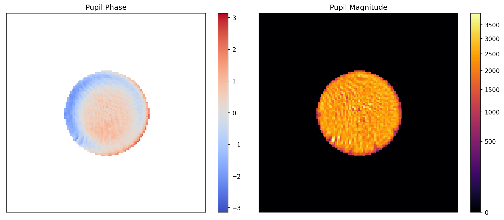
Below is a plot of the phase and magnitude of the retrieved pupil function from a PSF recorded from this instrument. To generate this plot we simply call the plot method of the PhaseRetrievalResult object (in this case pr_result).
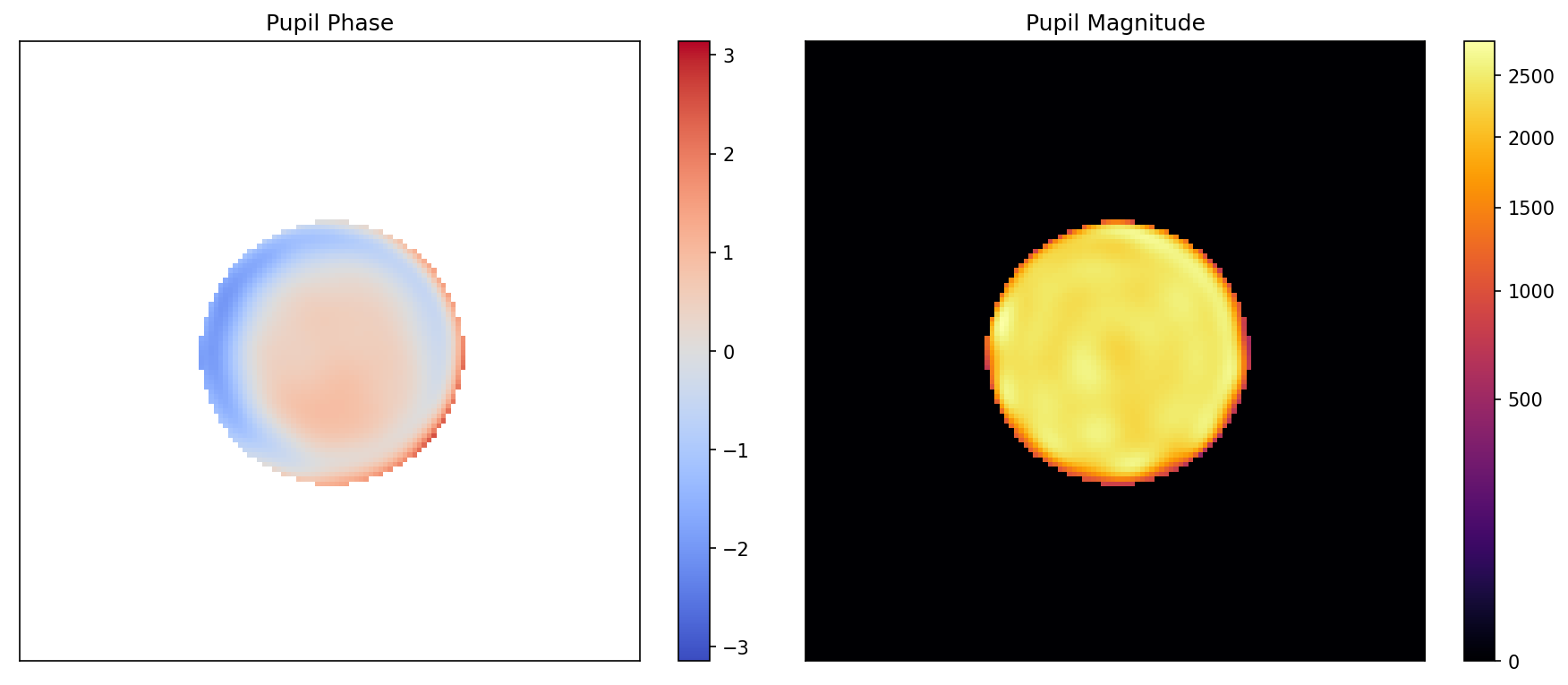
And here the phase and magnitude have been fitted to 120 zernike polynomials. To generate this plot we simply call the plot method of the ZernikeDecomposition object (in this case pr_result.zd_result).
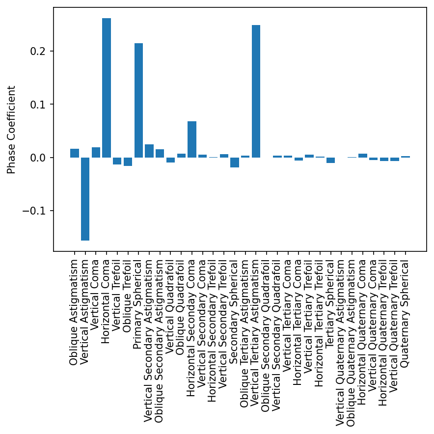
We can plot the magnitude of the first 15 named phase coefficients by calling pr_result.zd_result.plot_named_coefs().
NOTE: If all that is needed is phase, e.g. for adaptive optical correction, then most normal ways of estimating the background should be sufficient and you can use the phase_only keyword. However, if you want to properly model your PSF for something like deconvolution then you should be aware that the magnitude estimate is incredibly sensitive to the background correction applied to the data prior to running the algorithm, and multiple background methods/parameters should be tried.
zernike.py
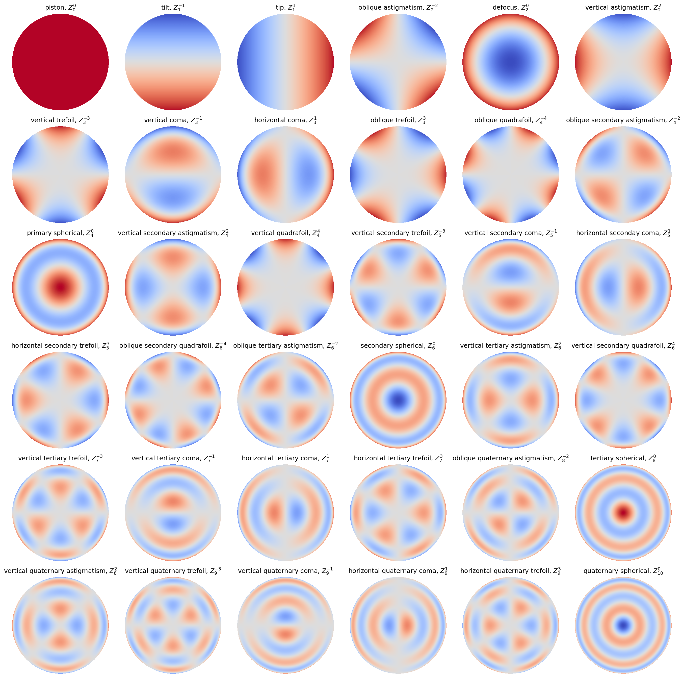
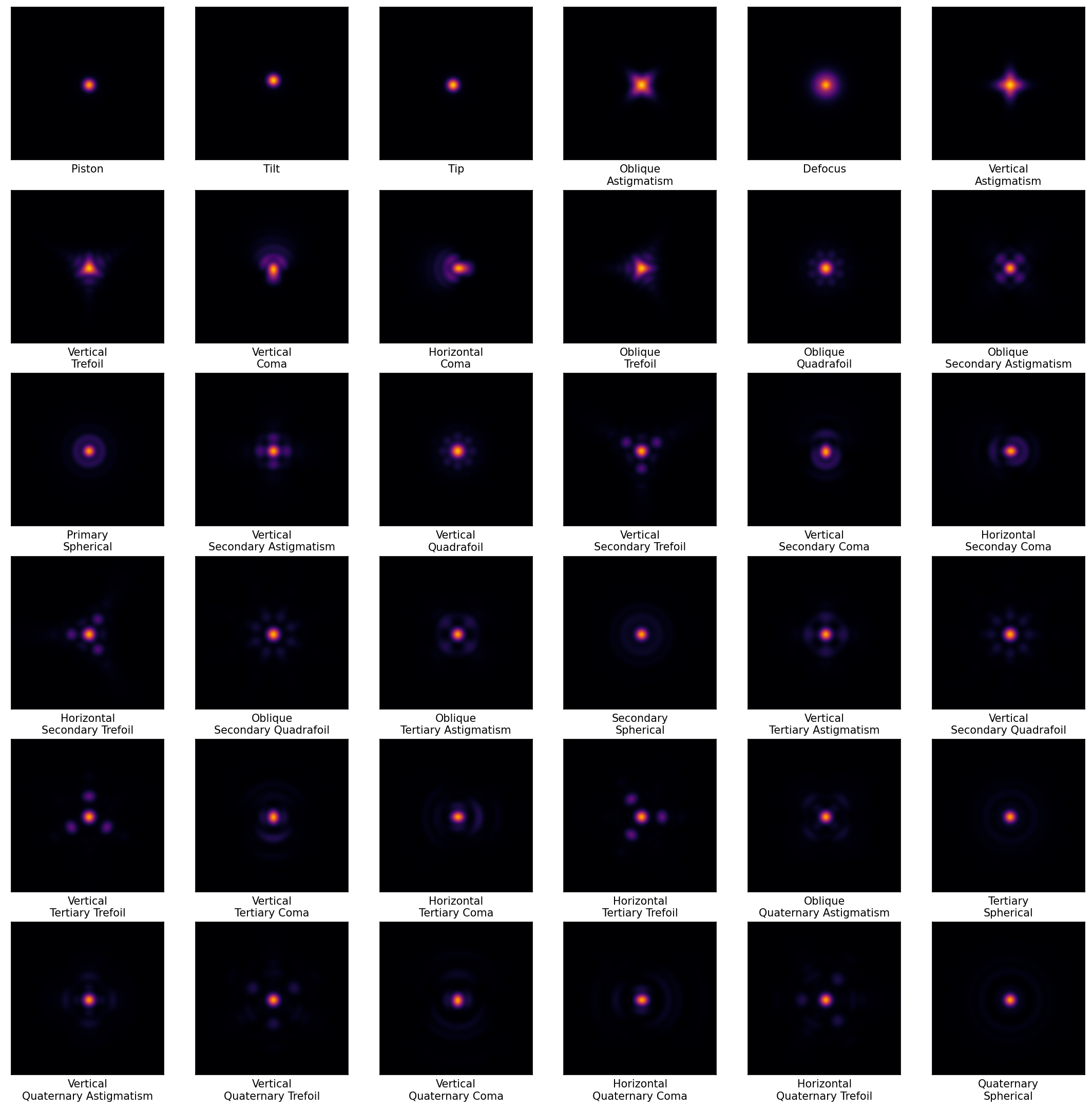
Zernike Polynomials are orthonormal functions defined over the unit disk. Being orthonormal any function defined on a unit disk has a unique decomposition into Zernike polynomials. In this package, the Zernike polynomials are used to quantify the abberation of the phase and magnitude of the retrieved back pupil of the optical system. To do so one can call the fit_to_zernikes method of a PhaseRetrievalResult object, which will fit a specified number of Zernike modes to the back pupil's retrieved phase and magnitude, each independently, and return a ZernikeDecomposition object. The ZernikeDecomposition that is returned is also saved as an attribute of the PhaseRetreivalResult object on which the fit_to_zernikes method was called, for convenience. ZernikeDecomposition objects have plotting methods so that the user can inspect the decomposition. ZernikeDecomposition objects also have methods for reconstructing the phase, magnitude or complete complex pupil which can be fed back into HanserPSF to generate an abberated, but noise free, PSF. The method for doing this simply is currently a member of the PhaseRetreivalResult class but will probably be moved to the ZernikeDecomposition class later.
utils.py
Most of the contents of utils won't be useful to the average user save one function: prep_data_for_PR(data, xysize=None, multiplier=1.5). prep_data_for_PR can, as its name suggests, be used to quickly prep PSF image data for phase retrieval using the retrieve_phase function of the phase_retrieval module.
LabVIEW API
An example of inputing a 3D stack and running this python function from LabVIEW (>2018) is given in \labview\Test Phase Retrieval.vi
References
Release history Release notifications | RSS feed


Download files
Download the file for your platform. If you're not sure which to choose, learn more about installing packages.
Source Distribution
Built Distribution
Filter files by name, interpreter, ABI, and platform.
If you're not sure about the file name format, learn more about wheel file names.
Copy a direct link to the current filters
File details
Details for the file pyotf-0.0.3.tar.gz.
File metadata
- Download URL: pyotf-0.0.3.tar.gz
- Upload date:
- Size: 53.6 kB
- Tags: Source
- Uploaded using Trusted Publishing? No
- Uploaded via: twine/4.0.1 CPython/3.9.13
File hashes
| Algorithm | Hash digest | |
|---|---|---|
| SHA256 |
78ca6efcfa575894a93661ebbc5e602dc83d083620d62f925ccbd1c1dc2d7b27
|
|
| MD5 |
ebc83499faa47854fadd75e8cdecac95
|
|
| BLAKE2b-256 |
2aac550d946e0ac13a680a9b104d389bdbc920741c84a4c62ab4710d0be46d74
|
File details
Details for the file pyotf-0.0.3-py3-none-any.whl.
File metadata
- Download URL: pyotf-0.0.3-py3-none-any.whl
- Upload date:
- Size: 39.2 kB
- Tags: Python 3
- Uploaded using Trusted Publishing? No
- Uploaded via: twine/4.0.1 CPython/3.9.13
File hashes
| Algorithm | Hash digest | |
|---|---|---|
| SHA256 |
1eb74e2b551f76b5604f21cef3511421a64c49a31022cca16cd3ef81c2d0a5cf
|
|
| MD5 |
2cc5685e43d3f3c54bb3fd2f987acd1f
|
|
| BLAKE2b-256 |
2c59ec7d4320f20146a90f754e58dcda7471e634539788408fafcbfb1a9683e0
|


