Python implementation for Spline-based Abel Transform

Project description
pySAT - Python Implementation for Spline-based Abel Transform
Context
In combustion research, optical diagnostics often necessitate Abel inversion to deconvolve the measurements of axisymmetric flames, especially to determine local soot temperature fields from integrated flame radiative emission measurements. However, traditional Abel inversion methods can considerably amplify experimental noise, especially towards the flame centerline. Although various strategies exist to mitigate this issue, they typically do not address the correction of signal trapping within the flame. In this context, pySAT is developed as an alternative without noise amplification, capable of correcting the signal trapping effect in different flame configurations.
Theoretical description
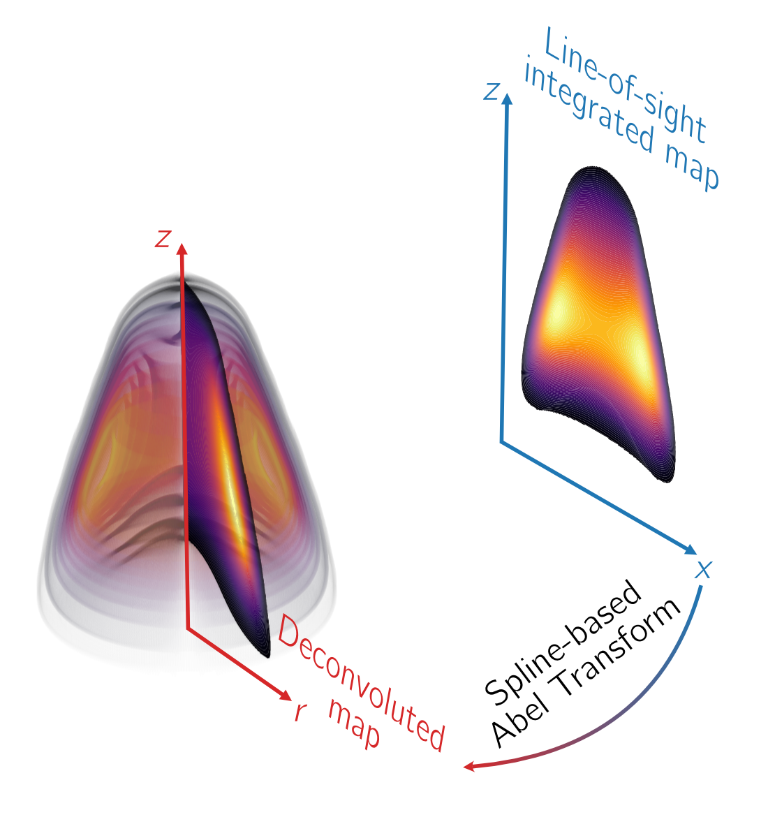
The Abel integral equation is mathematically formulated as follows: $$ S(x) = 2 \int_{x}^{\infty} \frac{\kappa(r) F(x, r)}{\sqrt{r^{2} - x^{2}}}~r dr. $$ The line-of-sight integrated signal $S(x)$ is known and the task is the determination of the deconvoluted $\kappa(r)$. Here, $\kappa(r)$ is assumed as a cubic spline. A cubic spline is a function that is defined by $N-1$ cubic polynomials $\kappa_{i}(r)$. Knots must to me defined and may be irregularly distributed.
Due to the continuous and differentiable nature of $S(x)$, clamped condition is imposed by setting null-derivative at the endpoints, and a null value at the end of the domain. Also, as it is not possible to obtain negative reconstructions from the projected values, a non-negativity constraint is imposed at the knots.
The direct Abel transform of this spline based profile leads to a model signal $S_{mod}$. Being a cubic spline, the values of the knots $\kappa_{i}$ are determined through the following minimization problem:
$$ \arg\min_{\kappa} \left[ \int \left[S_{\text{mod}}(x, \kappa_{1}, \dots, \kappa_{N}) - S_{exp}(x) \right]^{2} + \mu \int_{0}^{R}\kappa^{\prime \prime}(r)^{2}~dr\right] $$
Line-of-sight attenuation (LOSA)
In LOSA measurements, the transmissivity $S(x) = -\ln{\tau(x)}$ is measured to retrieve the extinction coefficient $\kappa(r) = \kappa_{ext}(r)$.
$$ \tau(x) = \frac{I(x)}{I_{0}(x)} = \exp{\left(-2\int_{x}^{\infty} \frac{\kappa_{ext}(r)}{\sqrt{r^{2} - x^{2}}}~rdr\right)}, $$ where $I(x)$ and $I_{0}(x)$ is the light intensity after and before passing through the sooting medium, respectively. Because attenuation is what it is measured, self-absorption has not to be corrected ($F(x, r) = 1$).
Soot Spectral Emission (SSE)
Emission measures line-of-sight (LoS) integrated flame emission $S_{emi}(x)$ to retrieve local thermal emission rate $J(r)$:
$$ S_{emi}(x) = \int_{x}^{\infty} \frac{J(r) F(x, r)}{\sqrt{r^{2} - x^{2}}}~rdr. $$
Signal trapping model
Soot particles have the ability to scatter and absorb light, leading to the attenuation of photon intensity along the LoS from the flame to the detector. When this effect is considered, a correction factor has to be defined. This one lies on the extinction profile (retrieved from LOSA). The correction $F$ has to be computed for each position in the flame: $$ F(x_{s}, y_{s}) = \exp{-\left(\int_{D}^{\infty} \kappa_{ext}(r)~dy\right)} $$
Example
The synthetic transmissivity and line-of-sight integrated emission data are located in the data_test folder emulating a measurements campaign of LOSA and SSE. In the demo.ipynb file, an application of the Spline-based Abel Transform (pySAT) is performed on the synthetic data. The steps are the following:
- Perform the Abel inversion on the transmissivity to retrieve $\kappa_{ext}$. The result of this process can be also the signal trapping factor $F$.
- To deconvolute the line-of-sight integrated emission, the signal trapping factor $F$ could be used or not. Since the extinction is available, then the trapping is corrected.
Installation
Conda
If you are more familiar with conda, it is strongly recommended to create an environment to isolate this tool from any other. Even so, the package will be installed via PIP. We are working to include it in conda-forge.
To create the environment, open a terminal and run:
conda create --name pysat-env
To activate the envinroment (now and every time you want to use pySAT):
conda activate pysat-env
To install the package:
pip install pysat-abel
PIP
It is also recomended to use a python virtualenv for your project. Open a terminal in the folder you want to work and type:
python -m venv pysat-env
You'll have to activate it (now and every time you want to use pySAT):
source pysat-env/bin/activate
To install the package:
pip install pysat-abel
Release history Release notifications | RSS feed


Download files
Download the file for your platform. If you're not sure which to choose, learn more about installing packages.
Source Distribution
Built Distribution
Filter files by name, interpreter, ABI, and platform.
If you're not sure about the file name format, learn more about wheel file names.
Copy a direct link to the current filters
File details
Details for the file pysat_abel-0.1.3.tar.gz.
File metadata
- Download URL: pysat_abel-0.1.3.tar.gz
- Upload date:
- Size: 24.2 kB
- Tags: Source
- Uploaded using Trusted Publishing? No
- Uploaded via: twine/6.1.0 CPython/3.12.4
File hashes
| Algorithm | Hash digest | |
|---|---|---|
| SHA256 |
16ae342d9b554d6dff9956880c75460a980effd6a40490c66dfa754ebc63c2ac
|
|
| MD5 |
1cd03cfbcce5ecc0f5350916372f1664
|
|
| BLAKE2b-256 |
7131833948dd4ae797a1a966d35d2fe614603d88c7fb76202c41e50e16e78da6
|
File details
Details for the file pysat_abel-0.1.3-py3-none-any.whl.
File metadata
- Download URL: pysat_abel-0.1.3-py3-none-any.whl
- Upload date:
- Size: 22.1 kB
- Tags: Python 3
- Uploaded using Trusted Publishing? No
- Uploaded via: twine/6.1.0 CPython/3.12.4
File hashes
| Algorithm | Hash digest | |
|---|---|---|
| SHA256 |
34b5f0ba5d495c42af107b070a681cc3b000c85a70a7eb41c9e38b26932ecac1
|
|
| MD5 |
c637e1cbe85ee62ee5e60e663e6f0f77
|
|
| BLAKE2b-256 |
39a00b5417d5e27c27ddc3e607bbc75fd5763ddb7f78ffda9f8ff86d34b56336
|


