pytissueoptics 1.0.4

Tissue optics Monte Carlo

Light propagation with Monte Carlo in Python

This is an extremely simple object-oriented code in Python that simulates the propagation of light in scattering tissue. It is not just simple: it is outrageously simple and very slow (see below). However, it is extremely easy to understand and most importantly very simple modify. It is a Python implementation of Monte Carlo, as beautifully illustrated by the standard, tested, and loved MCML from Wang, Jacques and Zheng , itself based on Prahl and completely documented, explained, dissected by Jacques and Prahl. Everyone is doing Monte Carlo in tissue, and nothing would be possible without the work of these pionneers.

It may be slow, but speed is more than code performance: anyone with little to no experience can simulate something instantly instead of having to understand C, C++ or, god forbid, GPU code. Therefore, you can quickly modifiy everything in an afternoon and get your results in a few hours, instead of learning C (a few weeks?), learn to work with compiled code (a few days? libraries anyone?) and finally modify the C code written by someone else (days? weeks?). I think the overall speed to be concerned about is "the time it takes to get an answer", not necessarily "the time it takes to run 100,000 photons". Considering many calculations with high performance code (in C for instance) take a few minutes, it is fairly reasonable to imagine you could start a calculation in Python, run it overnight and get an answer the next day after a few hours of calculations. I think there is a need for such a solution, and you will find it here.

Therefore, the whole point is the following: this code is perfect for quickly prototyping a small calculation, and then determine if you need performance or not. For many things, you actually don't.

Getting started

Install with pip or get the code from GitHub. You can run the example code immediately:

pip install pytissueoptics --upgrade
python -m pytissueoptics

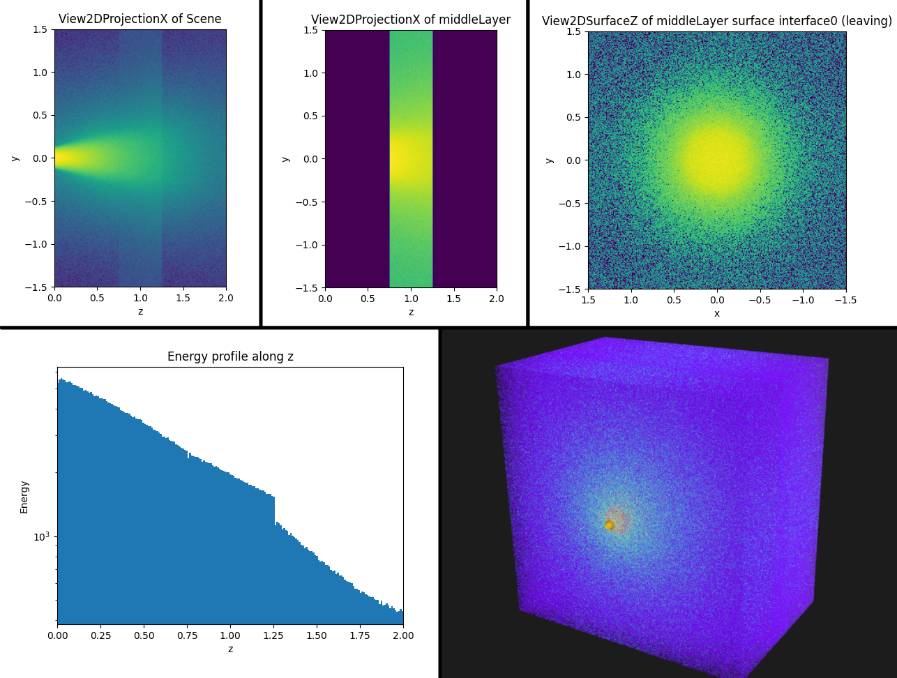
You need Python 3, it will not work with Python 2. The example code will show you a graph of the energy deposited in the plane xz from a isotropic source at the origin:

Then it will display the logarithm (log10) of the intensity as a fonction of distance along the x direction:

We can also display the intensity on surfaces:

Then, the idea would be to modify the code for your geometry (layers, boxes, cubes, spheres, etc...) and compute what you want.

What it can do

There are 6 main concepts (or Class in object-oriented language) in this code:

1. Photon: The photon is the main actor: it has a position, it propagates in a given direction. Its direction is changed when it scatters. It does not know anything about geometry or physical properties of tissue.
2. Source: A group of photons, such as IsotropicSource, PencilSource with specific properties. You provide the characteristics you want and it will give you a list of photons that responds to these criteria. This list of photons will give you the answer you want after it has propagated in the Object of interest.
3. Material: The scattering properties and the methods to calculate the scattering angles are the responsibility of the Material class. The Material also knows how to move the photon between two points (for instance, if there is birefringence, this is where you would put it although polarization is currently not implemented).
4. Geometry: A real-world geometry (Box, Cube, Sphere, Layer, etc...). The geometry has two important variables: a Material (which will dictate its optical properties i.e. scattering and index) and a Stats object to keep track of physical values of interest. The material will provide the required functions to compute the scattering angles, and the photon will use these angles to compute its next position. The Stats object will compute the relevant statistics.
5. Stats: An object to keep track of something you want. For now, it keeps track of volumetric quantities (i.e. the energy deposited in the tissue) and intensities through the surfaces delimiting geometries.
6. Finally, very useful Vector, UnitVector and Surface helper classes with their subclasses are used to simplify any 3D computation with vectors, planes, surfaces, because they can be used like other values (they can be added, subtracted, normalized, etc...).

Limitations

There are many limitations, as this is mostly a teaching tool, but I use it for real calculations in my research:

1. It really is not fully tested yet as of 1.0.4, especially with reflections. Setting all indices to 1.0 is a safe measure to get safe results (but obviously without reflections).
2. It only uses Henyey-Greenstein because it is sufficient most of the time.
3. Documentation is sparse at best.
4. You have probably noticed that the axes on the graphs are currently not labelled. Don't tell my students.
5. Did I say it was slow? It is approximately 50x slower than the well-known code MCML on the same machine. I know, and now I know that you know, but see Advantages below.

Advantages

However, there are advantages:

1. It is extremely simple to understand.
2. The code is very clear with only a few files in a single directory.
3. It can be used for teaching tissue optics.
4. It can be used for teaching object-oriented programming for those not familiar with it.
5. It is fairly easy to modify for your own purpose. Many modifications do not even require to subclass.
6. In addition, because it is very easy to parallelize a Monte Carlo calculations (all runs are independant), splitting the job onto several CPUs is a good option to gain a factor of close to 10 in perfromance on many computers. I have not done it yet.

The core of the code

The code is in fact so simple, here is the complete code that can create graphs similar to the ones above in 10 seconds on my computer:

from pytissueoptics import *

# We choose a material with scattering properties
mat    = Material(mu_s=30, mu_a = 0.1, g = 0.8, index = 1.4)

# We want stats: we must determine over what volume we want the energy
stats  = Stats(min = (-2,-2,-2), max = (2,2,2), size = (50,50,50))

# We pick a light source
source = PencilSource(direction=UnitVector(0,0,1), maxCount=10000)

# We pick a geometry
tissue = Layer(thickness=1, material=mat, stats=stats)

# We propagate the photons from the source inside the geometry
World.place(source, position=Vector(0,0,-1))
World.place(tissue, position=Vector(0,0,0))

World.compute(graphs=True)

# Report the results for all geometries
World.report()

The main function where the physics is hidden is Geometry.propagate(). World.compute() is a helper to call the function several times, and could possibly be parallelized:

class Geometry:
  [...]

    def propagate(self, photon):
        photon.transformToLocalCoordinates(self.origin)
        self.scoreWhenStarting(photon)
        d = 0
        while photon.isAlive and self.contains(photon.r):
            # Pick distance to scattering point
            if d <= 0:
                d = self.material.getScatteringDistance(photon)

            distToPropagate, surface = self.nextExitInterface(photon.r, photon.ez, d)

            if surface is None:
                # If the scattering point is still inside, we simply move
                # Default is simply photon.moveBy(d) but other things 
                # would be here. Create a new material for other behaviour
                self.material.move(photon, d=d)
                d = 0
                # Interact with volume: default is absorption only
                # Default is simply absorb energy. Create a Material
                # for other behaviour
                delta = self.material.interactWith(photon)
                self.scoreInVolume(photon, delta)

                # Scatter within volume
                theta, phi = self.material.getScatteringAngles(photon)
                photon.scatterBy(theta, phi)
            else:
                # If the photon crosses an interface, we move to the surface
                self.material.move(photon, d=distToPropagate)

                # Determine if reflected or not with Fresnel coefficients
                if self.isReflected(photon, surface): 
                    # reflect photon and keep propagating
                    photon.reflect(surface)
                    photon.moveBy(d=1e-3) # Move away from surface
                    d -= distToPropagate
                else:
                    # transmit, score, and leave
                    photon.refract(surface)
                    self.scoreWhenCrossing(photon, surface)
                    photon.moveBy(d=1e-3) # We make sure we are out
                    break

            # And go again    
            photon.roulette()

        # Because the code will not typically calculate millions of photons, it is
        # inexpensive to keep all the propagated photons.  This allows users
        # to go through the list after the fact for a calculation of their choice
        self.scoreWhenFinal(photon)
        photon.transformFromLocalCoordinates(self.origin)


[...]
class World:
  [...]
    @classmethod
    def compute(self, graphs):
        World.startCalculation()
        N = 0
        for source in World.sources:
            N += source.maxCount

            for i, photon in enumerate(source):
                while photon.isAlive:
                    currentGeometry = World.contains(photon.r)
                    if currentGeometry is not None:
                        currentGeometry.propagate(photon)
                    else:
                        distance, surface, nextGeometry = World.nextObstacle(photon)
                        if surface is not None:
                            # Moving to next object in air
                            photon.moveBy(distance)
                            R = photon.fresnelCoefficient(surface)
                            photon.refract(surface)
                            photon.decreaseWeightBy(R*photon.weight)
                            photon.moveBy(1e-4)
                        else:
                            photon.weight = 0

                World.showProgress(i+1, maxCount=source.maxCount, graphs=graphs)

        duration = World.completeCalculation()
        print("{0:.1f} ms per photon\n".format(duration*1000/N))

Note that this propagate function is part of the Geometry object and does not make any assumption on the details of the geometry, and relies on whatever material was provided to get the scattering angles.

How to go about modifying for your own purpose

1. Maybe you have a special light source?

   1. Subclass Source with your own light source and compute the photon properties in newPhoton according to your own rules. Use your source instead of IsotropicSource in the example above:

      class MySource(Source):
           def __init__(self, myProperty, position, maxCount):
               super(MySource, self).__init__(position, maxCount)
               self.myProperty = myProperty
      
           def newPhoton(self) -> Photon:
               p = Photon()
               # Do your thing here with self.myProperty and modify p
               return p
      

2. Maybe you have a special material scattering model?

   1. Subclass Material and override the methods for getScatteringAngles(). Use your material in your geometry instead of Material in the example above. You could use the photon direction, polarization, position, or even its wavelength to compute its scattering angles:

      class FunkyMaterial(Material):
           def __init__(self, myProperty, mu_s = 0, mu_a = 0, g = 0):
               super(MySource, self).__init__(mu_s, mu_a, g)
               self.myProperty = myProperty
      
           def getScatteringAngles(self, photon) -> (float, float):
               # Do your thing here with self.myProperty and compute theta, phi
               # Use Photon if needed (position, direction, wavelength, etc..)
               return (theta, phi)
      

3. If photon.keepPathHistory() is called, it will keep track all positions during its lifetime. You can then compute whatever you want by rewriting that part of the code or with a hook function I will write at some point.

4. Maybe you want to compute some funky stats? At each step, scoreInVolume is called with the photon and the drop in energy at that step. When leaving the geometry through a surface, scoreWhenCrossing is called with the photon and the last position inside.

5. Maybe your have a special geometry? Subclass Geometry and override the contains method to compute whether or not a given position is inside your object or not, and intersection to compute the point on the surface of your object where the photon exits.