Trend detection in time series for risk management, drawdown analysis, and machine learning classification models.

Project description


pytrendseries is a Python library for detection of trends in time series like: stock prices, monthly sales, daily temperature of a city and so on.
The input data must be a pandas.DataFrame format containing one column as observed data (in float or int format). Follow example below:
import pandas as pd
data = pd.read_csv("tests/resource/stock_prices.csv")
filtered_data = data[['period','close']].set_index("period")
filtered_data.columns = ['close_price']
filtered_data.index = pd.to_datetime(filtered_data.index)
filtered_data = filtered_data.sort_index()
Once some trend is identified, pytrendseries provides period on trend, drawdown, maximum drawdown (or drawup in case of uptrend) and a plot with all trends found.
Installation
Using pip
You can install using the pip package manager by running:
pip install pytrendseries
Alternatively, you could install the latest version directly from Github:
python -m pip install git+https://github.com/rafa-rod/pytrendseries.git
Why pytrendseries is important?
Detection of trends could be used in machine learning algorithms such as classification problems like binary (1 = uptrend, 0 = otherwise) or non-binary classifications (1 = uptrend, -1 = downtrend, 0 = otherwise). Besides that, could be used in prediction problems.
Example
Inform:
- type of trend you desire to investigate => downtrend or uptrend;
- window or maximum period of a trend (example: 60 days considering 1 day as 1 period);
- the minimum value that represents the number of consecutive days (or another period of time) to be considered a trend (default 5 periods).
import pytrendseries

trend = "downtrend"
window = 126 #6 months

trends_detected = pytrendseries.detecttrend(filtered_data, trend=trend, window=window)
The variable trends_detected is a dataframe that contains the initial and end date of each trend, the prices of each date, time span of each trend and the drawdown of each trend. Let's see the first five rows of this dataframe:
| Peak Date           | Valley Date         |   Peak   |   Valley |   index_peak  |index_valley |   time_span |   drawdown |
|:--------------------|:--------------------|---------:|---------:|--------------:|------------:|------------:|-----------:|
| 2000-01-03 00:00:00 | 2000-01-31 00:00:00 |  5.90057 |  5.12252 |             0 |          19 |          19 |  0.131859  |
| 2000-03-09 00:00:00 | 2000-04-24 00:00:00 |  6.42701 |  5.02208 |            45 |          76 |          31 |  0.218597  |
| 2000-05-02 00:00:00 | 2000-05-11 00:00:00 |  5.53684 |  5.29352 |            81 |          88 |           7 |  0.0439456 |
| 2000-05-16 00:00:00 | 2000-05-24 00:00:00 |  5.59962 |  5.24807 |            91 |          97 |           6 |  0.0627803 |
| 2000-06-08 00:00:00 | 2000-06-15 00:00:00 |  6.30359 |  6.1646  |           108 |         113 |           5 |  0.0220487 |
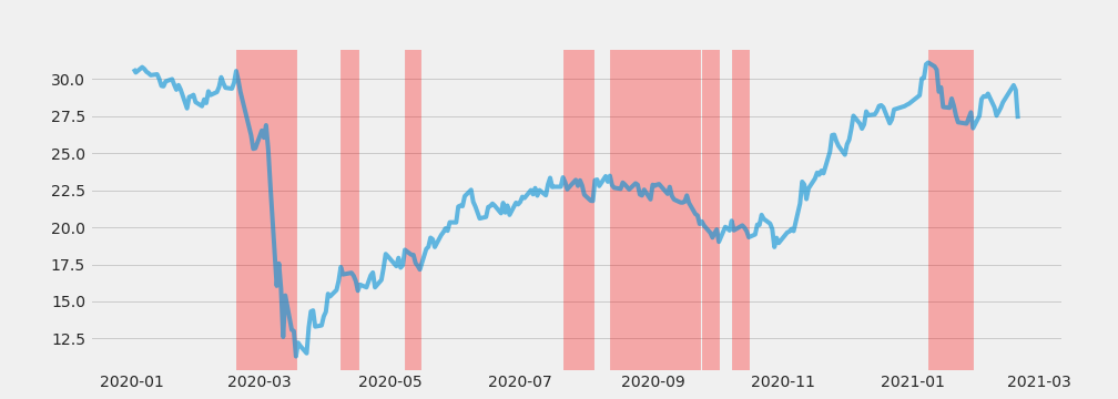
The easiest way to vizualize the trends detected, just call plot_trend function.
All trends detected, with maximum window informed and the minimum informed by the limit value, will be displayed.
import pytrendseries
trend = "downtrend"
window = 30
year = 2020

trends_detected = pytrendseries.detecttrend(filtered_data, trend=trend, window=window)
pytrendseries.vizplot.plot_trend(filtered_data, trends_detected, trend, year)
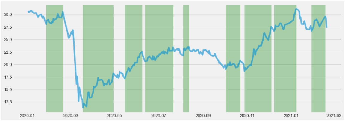
To visualize all uptrends found, inform trend='uptrend':
import pytrendseries
window = 30
year = 2020

trends_detected = pytrendseries.detecttrend(filtered_data, trend='uptrend', window=window)
pytrendseries.vizplot.plot_trend(filtered_data, trends_detected, 'uptrend', year)
Maximum Drawdown
The maxdrawdown calculates the Maximum Drawdown within non-overlapping time windows, providing detailed information about each significant drawdown event.
The maximum drawdown or maximum drawup can be obtained by sorting the dataframe by column drawdown. To do that, just code:
maxdd_in_window = trends_detected.sort_values("drawdown", ascending=False).iloc[0:1]
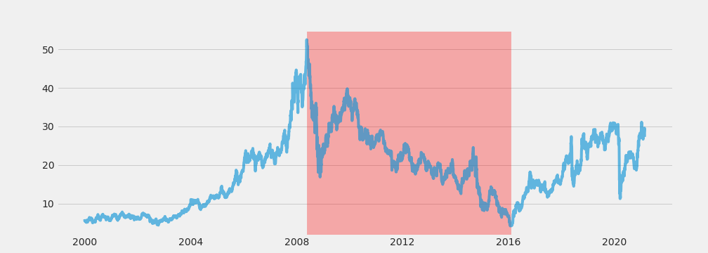
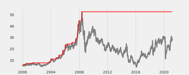
Another way is to call the function maxdrawdown. Note that this result will be differente once the maximum drawdown of the intire timeseries, unless you pass same window parameter.
maxdd = pytrendseries.maxdrawdown(filtered_data, window=None)
Output includes:
- Window Start/End dates;
- Peak and Valley dates with corresponding prices;
- Maximum Drawdown percentage;
- Time Span (number of periods from peak to valley).
You can code to vizualize as follows:
import matplotlib.pyplot as plt

plt.figure(figsize=(14,5))
plt.plot(filtered_data, alpha=0.6)
location_x = maxdd.values[:,0]
location_y = maxdd.values[:,1]
for i in range(location_x.shape[0]):
    plt.axvspan(location_x[i], location_y[i], alpha=0.3, color="red")
plt.grid(axis='x')
plt.show()
You may pass the parameter window to obtain the same result:
maxdd_in_window = pytrendseries.maxdrawdown(filtered_data, window=252)
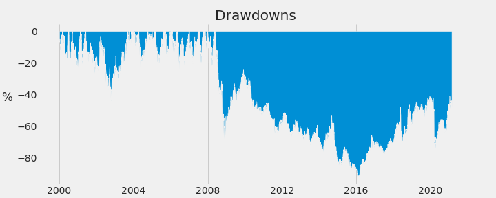
To vizualize all drawdowns of timeseries, call the following function:
import pytrendseries
pytrendseries.plot_drawdowns(filtered_data, figsize = (10,4), color="gray", alpha=0.6, title="Drawdowns", axis="y")
Another option is:
import pytrendseries
pytrendseries.plot_evolution(filtered_data, figsize = (10,4), colors=["gray", "red"], alphas=[1,0.6])
Current Drawdown
The calculate_current_drawdown function returns key metrics including the current price, last peak value and date, current drawdown percentage, and the duration (in number of records) since the last peak.
import pytrendseries
pytrendseries.calculate_current_drawdown(filtered_data)
Output example:
| current_price | last_peak | current_drawdown | last_peak_date | time_in_drawdown |
|---|---|---|---|---|
| 98.50 | 105.30 | -6.46% | 2024-01-15 | 12 |
Time Under Water (tuw)
To get time underwater (tuw), just type:
import pytrendseries
pytrendseries.calculate_time_under_water(filtered_data)
The output would be (showing the tail of the dataframe):
| Peak Date | Recovery Date |   Peak   |   Valley  |   MaxDD   | Time Underwater |   Status   |
|:----------|:--------------|---------:|----------:|----------:|----------------:|-----------:|
| 2007-12-28|   2008-05-06  | 44.66140 | 33.58194  |   0.24808 |       85        | Recovered  |
| 2008-05-06|   2008-05-09  | 45.00000 | 44.85000  |   0.00333 |        4        | Recovered  |
| 2008-05-13|   2008-05-15  | 46.95000 | 46.30000  |   0.01384 |        3        | Recovered  |
| 2008-05-21|      NaT      | 52.51000 |  4.20000  |   0.92002 |      235        |  Ongoing   |
The Status column indicates whether the drawdown period has recovered or is still ongoing, while Time Underwater shows the number of periods spent below the previous peak.
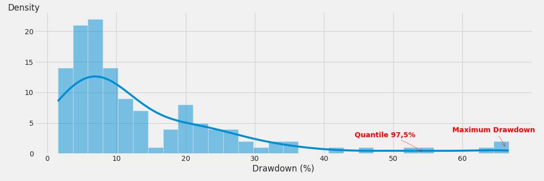
Another important usage of pytrendseries is to obtain the series of drawdowns or series of maximum drawdowns in order to calculate the drawdown at risk or maximum drawdown at risk.
import pytrendseries
import matplotlib.pyplot as plt
import seaborn as sns; sns.set_style("white")

trend = "downtrend"
window = 126 #6 months

trends_detected = pytrendseries.detecttrend(filtered_data, trend=trend, window=window)

plt.figure(figsize=(15,5))
sns.histplot(trends_detected["drawdown"]*100, kde=True, bins=30)
plt.ylabel("")
plt.box(False)
plt.annotate('Maximum Drawdown', xy=((trends_detected["drawdown"].max()-0.005)*100, 1),
             xycoords='data',
            xytext=(-105, 30), textcoords='offset points',color="red",
            weight='bold',
            arrowprops=dict(arrowstyle="->", color="r",
                            connectionstyle='arc3,rad=-0.1'))
plt.annotate('Quantile 97,5%', xy=((trends_detected["drawdown"].quantile(0.975)-0.005)*100, 0.2),
             xycoords='data',
            xytext=(-135, 30), textcoords='offset points',color="red",
            weight='bold',
            arrowprops=dict(arrowstyle="->", color="r",
                            connectionstyle='arc3,rad=-0.1'))
plt.xlabel("Drawdown (%)")
plt.ylabel("Density", rotation=0, labelpad=-30, loc="top")
plt.show()
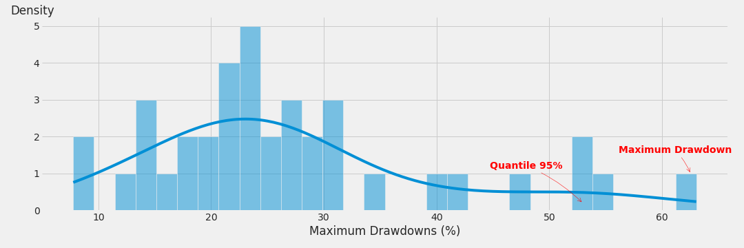
import pytrendseries
import matplotlib.pyplot as plt
import seaborn as sns; sns.set_style("white")

maxdd_in_window = pytrendseries.maxdrawdown(filtered_data, window=126)

plt.figure(figsize=(15,5))
sns.histplot(maxdd_in_window["MaxDD"]*100, kde=True, bins=30)
plt.ylabel("")
plt.box(False)
plt.annotate('Maximum Drawdown', xy=((maxdd_in_window["MaxDD"].max()-0.005)*100, 1),
             xycoords='data',
            xytext=(-105, 30), textcoords='offset points',color="red",
            weight='bold',
            arrowprops=dict(arrowstyle="->", color="r",
                            connectionstyle='arc3,rad=-0.1'))
plt.annotate('Quantile 95%', xy=((maxdd_in_window["MaxDD"].quantile(0.95)-0.005)*100, 0.2),
             xycoords='data',
            xytext=(-135, 50), textcoords='offset points',color="red",
            weight='bold',
            arrowprops=dict(arrowstyle="->", color="r",
                            connectionstyle='arc3,rad=-0.1'))
plt.xlabel("Maximum Drawdowns (%)")
plt.ylabel("Density", rotation=0, labelpad=-30, loc="top")
plt.show()
Trend Labeling for Machine Learning
The get_trends_labels function automates the process of labeling financial time series data based on detected market structures. By identifying peaks and valleys within a specified window, it segments the data into Uptrends, Downtrends, and No Trend periods.
Why use this for Machine Learning?
This function is particularly useful for supervised learning classification problems. Instead of trying to predict the exact future price (a regression problem), you can train models to predict the market state or direction.
- Target Variable Engineering: Converts raw price data into discrete classes (e.g.,
1,-1,0). - Noise Reduction: Ignores minor fluctuations by focusing on significant trends defined by the
windowandlimitparameters. - Flexibility: Allows custom labeling schemes (e.g., numeric for models, strings for interpretability).
Output Example
After running the function, your dataframe will include a new label column indicating the market regime for each date.
| Date | Close | Label | Market State |
|---|---|---|---|
| 2023-01-03 | 100.5 | 0 | No Trend |
| 2023-01-04 | 101.2 | 0 | No Trend |
| 2023-01-05 | 103.5 | 1 | Uptrend |
| 2023-01-06 | 105.0 | 1 | Uptrend |
| 2023-01-09 | 104.8 | 1 | Uptrend |
| 2023-01-10 | 102.0 | 0 | No Trend |
| 2023-01-11 | 99.5 | -1 | Downtrend |
| 2023-01-12 | 98.0 | -1 | Downtrend |
Usage Examples
1. Default Configuration
Uses standard numeric labels (1 for uptrend, -1 for downtrend, 0 for no trend).
import pytrendseries
df_labeled = pytrendseries.get_trends_labels(df, window=252, limit=5)
2. Custom String Labels
Useful for interpretability or specific model requirements.
custom_labels = {
    "uptrend": "BUY",
    "downtrend": "SELL",
    "notrend": "HOLD"
}
df_labeled = pytrendseries.get_trends_labels(df, labels=custom_labels)
3. Binary Classification (Uptrend vs. Rest)
Ignore downtrends and treat them as "no trend" for a specific strategy.
binary_labels = {
    "uptrend": 1,
    "notrend": 0
}
df_labeled = pytrendseries.get_trends_labels(df, labels=binary_labels)
Release history Release notifications | RSS feed


Download files
Download the file for your platform. If you're not sure which to choose, learn more about installing packages.
Source Distribution
Built Distribution
Filter files by name, interpreter, ABI, and platform.
If you're not sure about the file name format, learn more about wheel file names.
Copy a direct link to the current filters
File details
Details for the file pytrendseries-0.1.12.tar.gz.
File metadata
- Download URL: pytrendseries-0.1.12.tar.gz
- Upload date:
- Size: 18.5 kB
- Tags: Source
- Uploaded using Trusted Publishing? No
- Uploaded via: twine/6.2.0 CPython/3.12.10
File hashes
| Algorithm | Hash digest | |
|---|---|---|
| SHA256 |
4eaac554d371630459ac2815e449ee95940e0d4de1a363eb9fc6e4127d9fb585
|
|
| MD5 |
cf98e944e4fc42292aec1318111c9093
|
|
| BLAKE2b-256 |
5dd6bb8e820c59044e232528b34948cfae8ecde44417fc57c988f60e1d739e4f
|
File details
Details for the file pytrendseries-0.1.12-py3-none-any.whl.
File metadata
- Download URL: pytrendseries-0.1.12-py3-none-any.whl
- Upload date:
- Size: 17.6 kB
- Tags: Python 3
- Uploaded using Trusted Publishing? No
- Uploaded via: twine/6.2.0 CPython/3.12.10
File hashes
| Algorithm | Hash digest | |
|---|---|---|
| SHA256 |
eac0a17d6c27a830ba233e0d2365cbf1d0c852986ec1b046d49e3fa1111e26a0
|
|
| MD5 |
7b01741c38d3a7022600cf1d2f9ebd62
|
|
| BLAKE2b-256 |
fa9023b302db85a56e3039e947509e864f2d33c43f03dde0cfa42243d4a17c96
|


