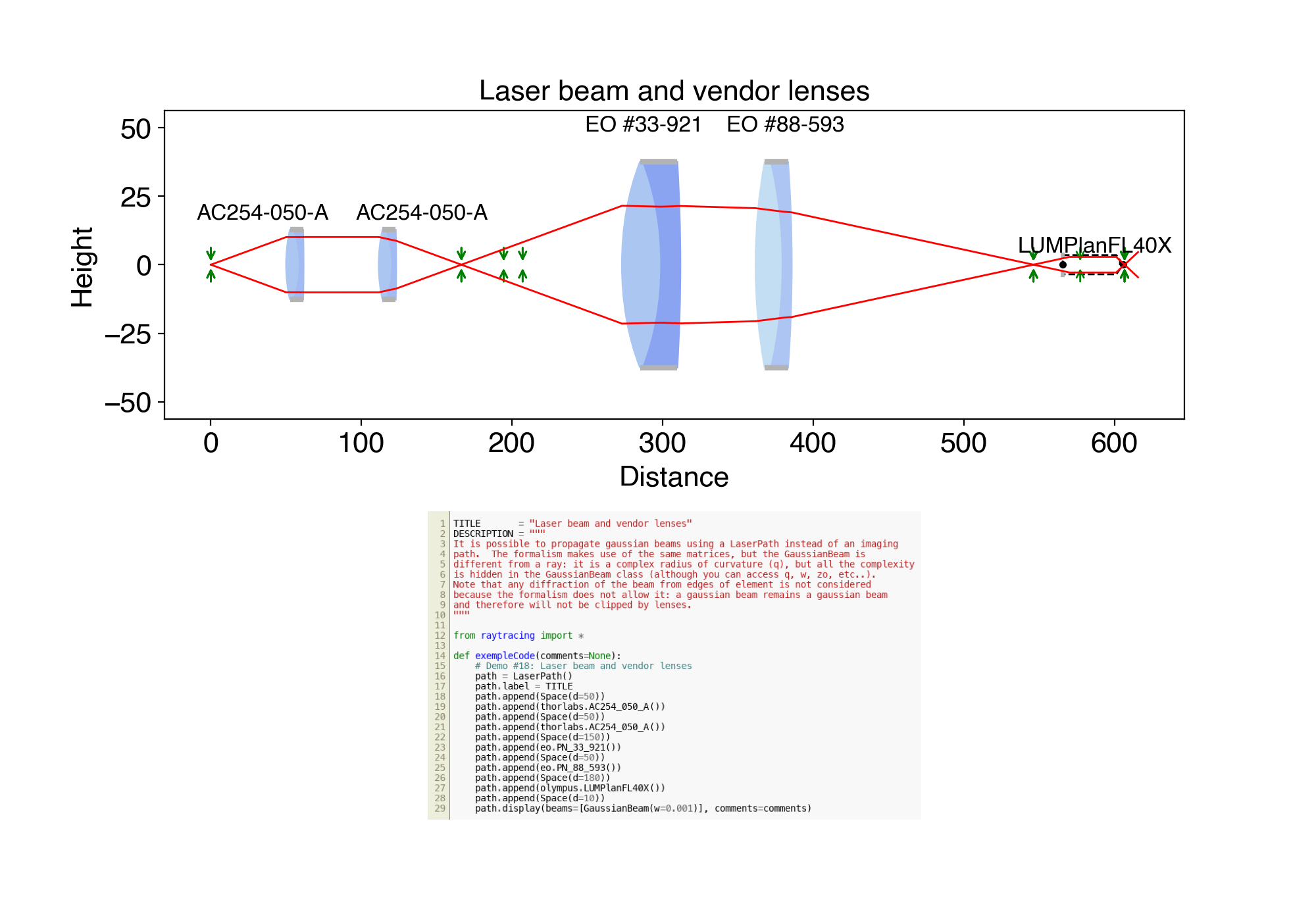
Simple optical ray tracing library to validate the design of an optical system.
Project description
RayTracing
by the DCC/M Lab group http://www.dccmlab.ca, guided by Prof. Daniel Côté.
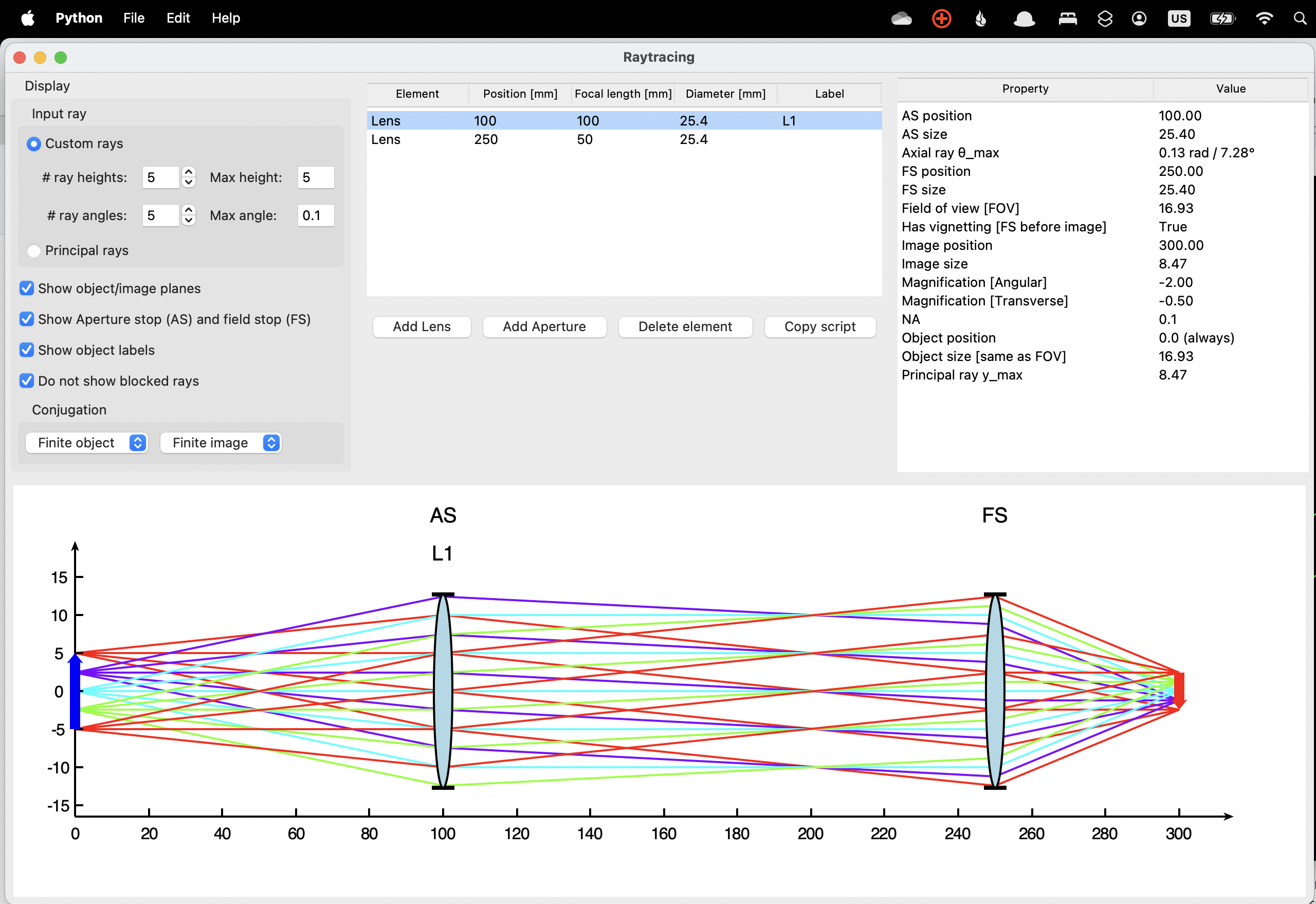
New: A graphical interface for Raytracing
A graphical interface is now available (macOS, Windows and Linux), with (python 3.12 and earlier, not 3.13):
pip install raytracing
python -m raytracing -a
This code aims to provide a simple ray tracing module for calculating various properties of optical paths (object, image, aperture stops, field stops). It makes use of ABCD matrices and does not consider spherical aberrations but can compute chromatic aberrations for simple cases when the materials are known. Since it uses the ABCD formalism (or Ray matrices, or Gauss matrices) it can perform tracing of rays and gaussian laser beams.
It is not a package to do "Rendering in 3D with raytracing".
The code has been developed first for teaching purposes and is used in my "Optique" Study Notes (french only), but also for actual use in my research. As of January 21st, 2021, there is an extensive, freely accessible, peer-reviewed tutorial in Journal of Neurophotonics:
"Tools and tutorial on practical ray tracing for microscopy"
by V. Pineau Noël*, S. Masoumi*, E. Parham*, G. Genest, L. Bégin, M.-A. Vigneault, D. C. Côté, Neurophotonics, 8(1), 010801 (2021). *Equal contributions. Permalink: https://doi.org/10.1117/1.NPh.8.1.010801
The published tutorial assumes version 1.3.x. There are video tutorials (in english or french, with english subtitles when in french) on YouTube. We have made no attempts at making high performance code but there is a GPU acceleration option through OpenCL and it still uses a python-like approach and hides the details, see below. Readability and simplicity of usage are the key here. It is a module with a few files, and only matplotlib and numpy as dependent modules.
Where do I get started?
- If you want to use the module, keep reading.
- If you have a suggestion or a bug report, go to Issues.
- If you want to read and contribute to the code, go to the Wiki for general considerations. We plan to have a roadmap in the near future.
Getting started
The module defines Ray , Matrix, MatrixGroup and ImagingPath as the main elements for tracing rays. Matrix and MatrixGroup are either one or a sequence of many matrices into which Ray will propagate. ImagingPath is also a sequence of elements, with an object at the front edge. Specific subclasses of Matrix exists: Space, Lens, ThicklLens, and Aperture. Finally, a ray fan is a collection of rays, originating from a given point with a range of angles.
We have tried to separate the calculation code (i.e. the matrices and subclasses) from the drawing code (figures and graphics). One can use the calculation code without any graphics calls.
If you want to perform calculations with coherent laser beams, then you use GaussianBeam and LaserPath. Everything is essentially the same, except that the formalism does not allow for the gaussian beam to be "blocked", hence any calculation of stops with aperture are not available in LaserPath. That part of the code is less developed, but it is nevertheless available.
What's new?
To get information about what is new, currently the best place is the release page on GitHub.
There is a Frequently Asked Questions page.
The article above is fully compatible with all 1.x versions starting at 1.3.
Installing and upgrading
You need matplotlib, which is a fairly standard Python module. If you do not have it, installing Anaconda is your best option. Python 3.6 or later is required. There are several ways to install the module:
- Simplest:
pip install raytracingorpip install --upgrade raytracing- If you need to install
pip, download getpip.py and run it withpython getpip.py
- If you need to install
- If you download the source of the module, then you can type:
python setup.py install - From GitHub, you can get the latest version (including bugs, which are 153% free!) and then type
python setup.py install - If you are completely lost, copying the folder
raytracing(the one that includes__init__.py) from the source file into the same directory as your own script will work. - Watch the tutorial with subtitles here.
Getting started
The simplest way to import the package in your own scripts after installing it:
from raytracing import *
This will import Ray , GaussianBeam, and several Matrix elements such as Space, Lens, ThickLens, Aperture, DielectricInterface, but also MatrixGroup (to group elements together), ImagingPath (to ray trace with an object at the front edge), LaserPath (to trace a gaussian laser beam from the front edge) and a few predefined other such as Objective (to create a very thick lens that mimicks an objective).
You create an ImagingPath or a LaserPath, which you then populate with optical elements such as Space, Lens or Aperture or vendor lenses. You can then adjust the path properties (object height in ImagingPath for instance or inputBeam for LaserPath) and display in matplotlib. You can create a group of elements with MatrixGroup for instance a telescope, a retrofocus or any group of optical elements you would like to treat as a "group". The Thorlabs and Edmund optics lenses, for instance, are defined as MatrixGroups.
This will show you a list of examples of things you can do (more on that in the Examples section):
python -m raytracing -l           # List examples
python -m raytracing -e all       # Run all of them
python -m raytracing -e 1,2,4,6   # Only run 1,2,4 and 6
python -m raytracing -t           # Run all the tests.  Some performance tests can take up to a minute, but they should all pass.
or request help with:
python -m raytracing -h
In your code, you would do this:
from raytracing import *

path = ImagingPath()
path.append(Space(d=50))
path.append(Lens(f=50, diameter=25))
path.append(Space(d=120))
path.append(Lens(f=70))
path.append(Space(d=100))
path.display()
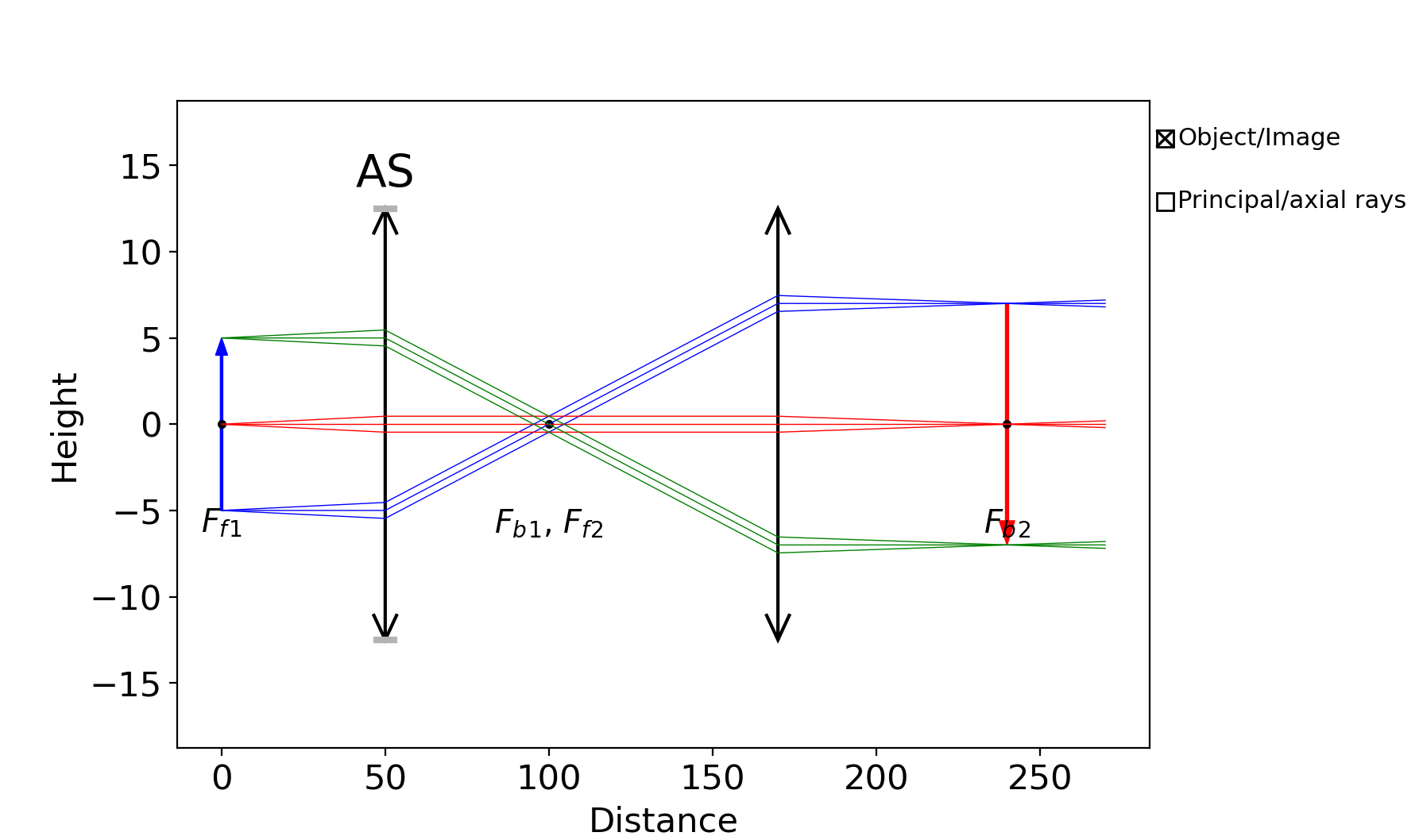
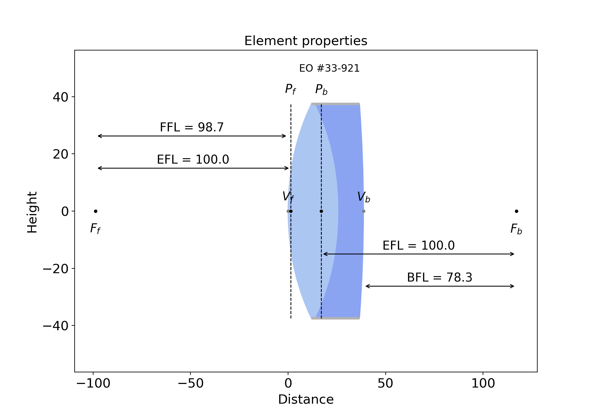
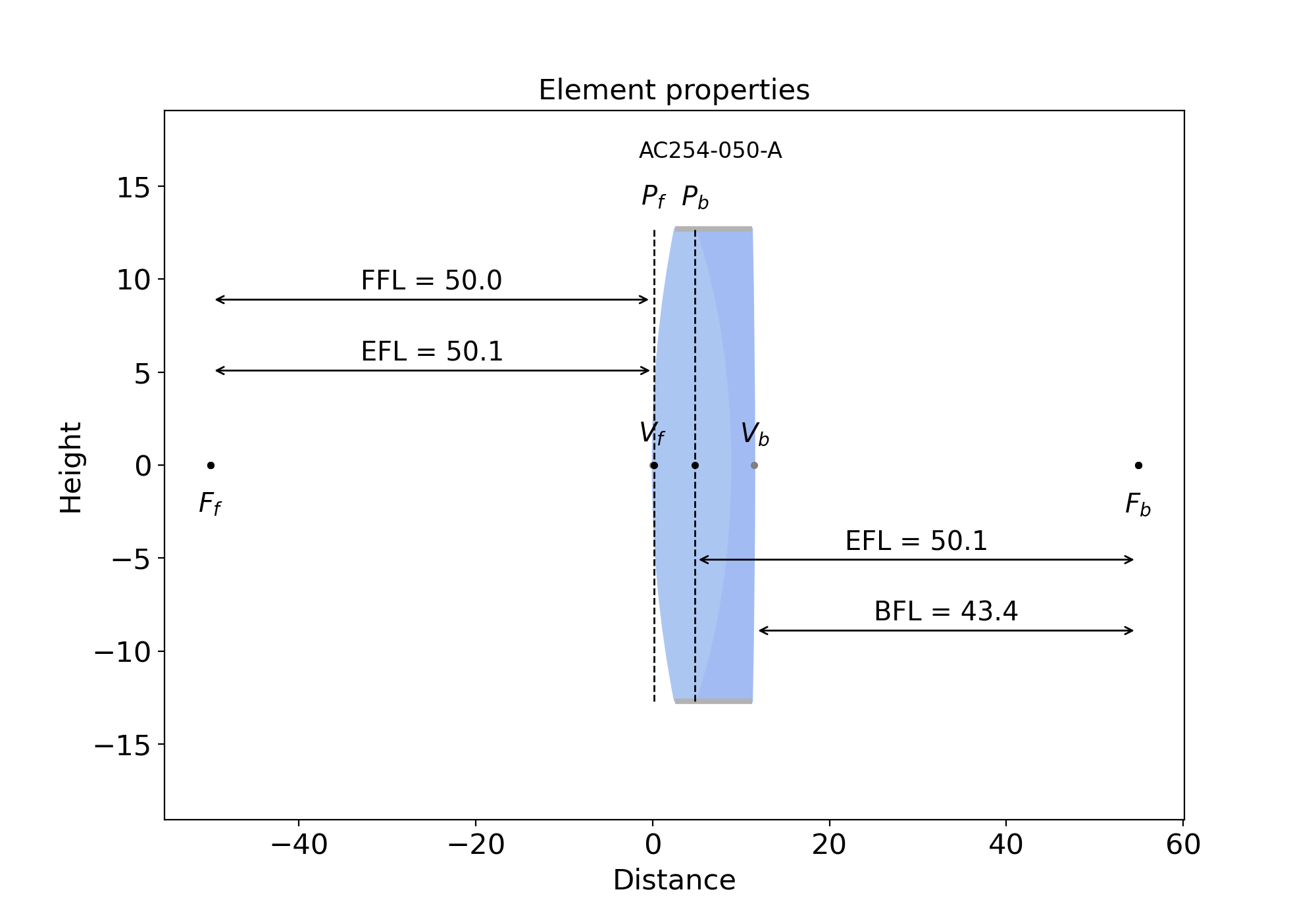
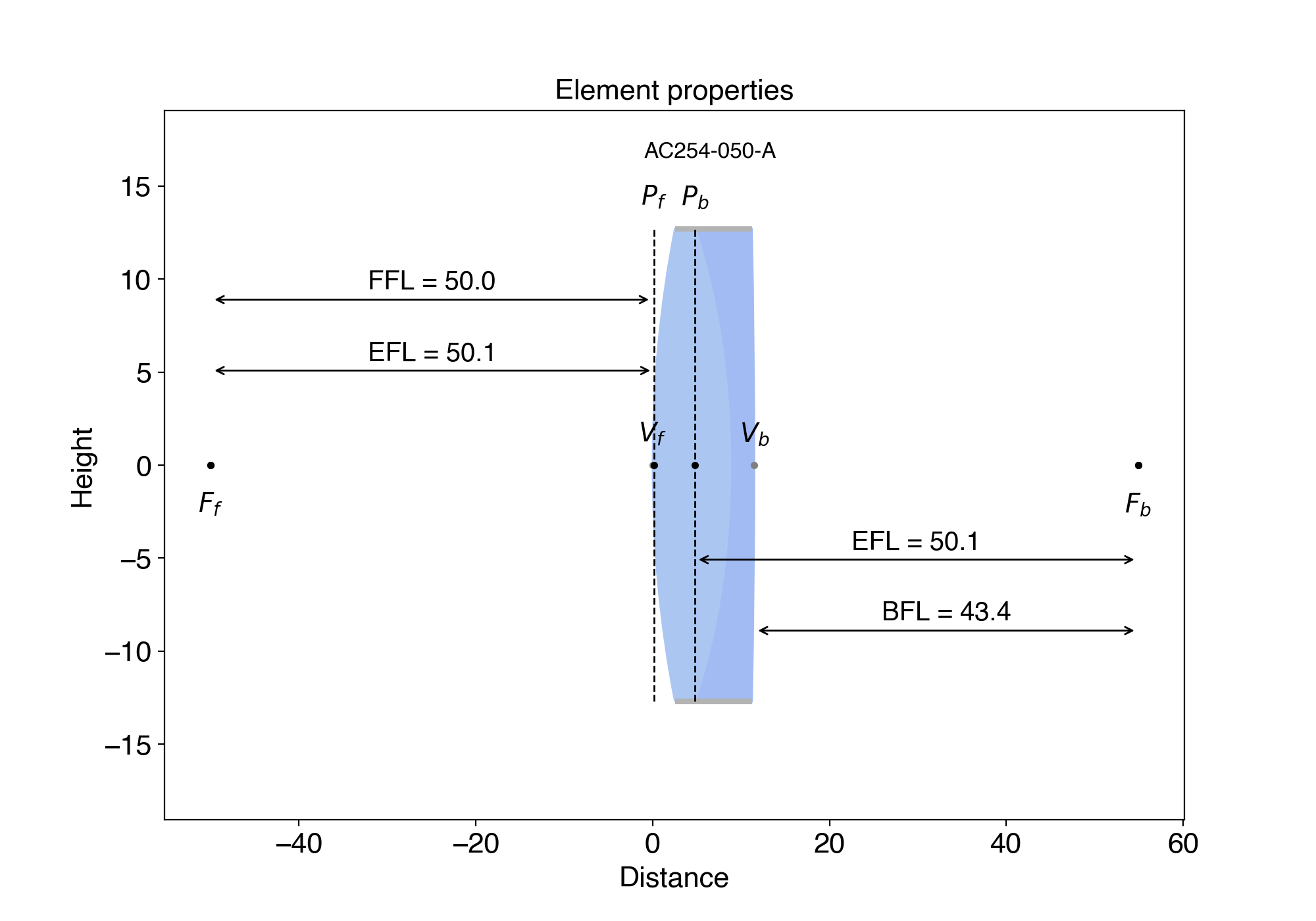
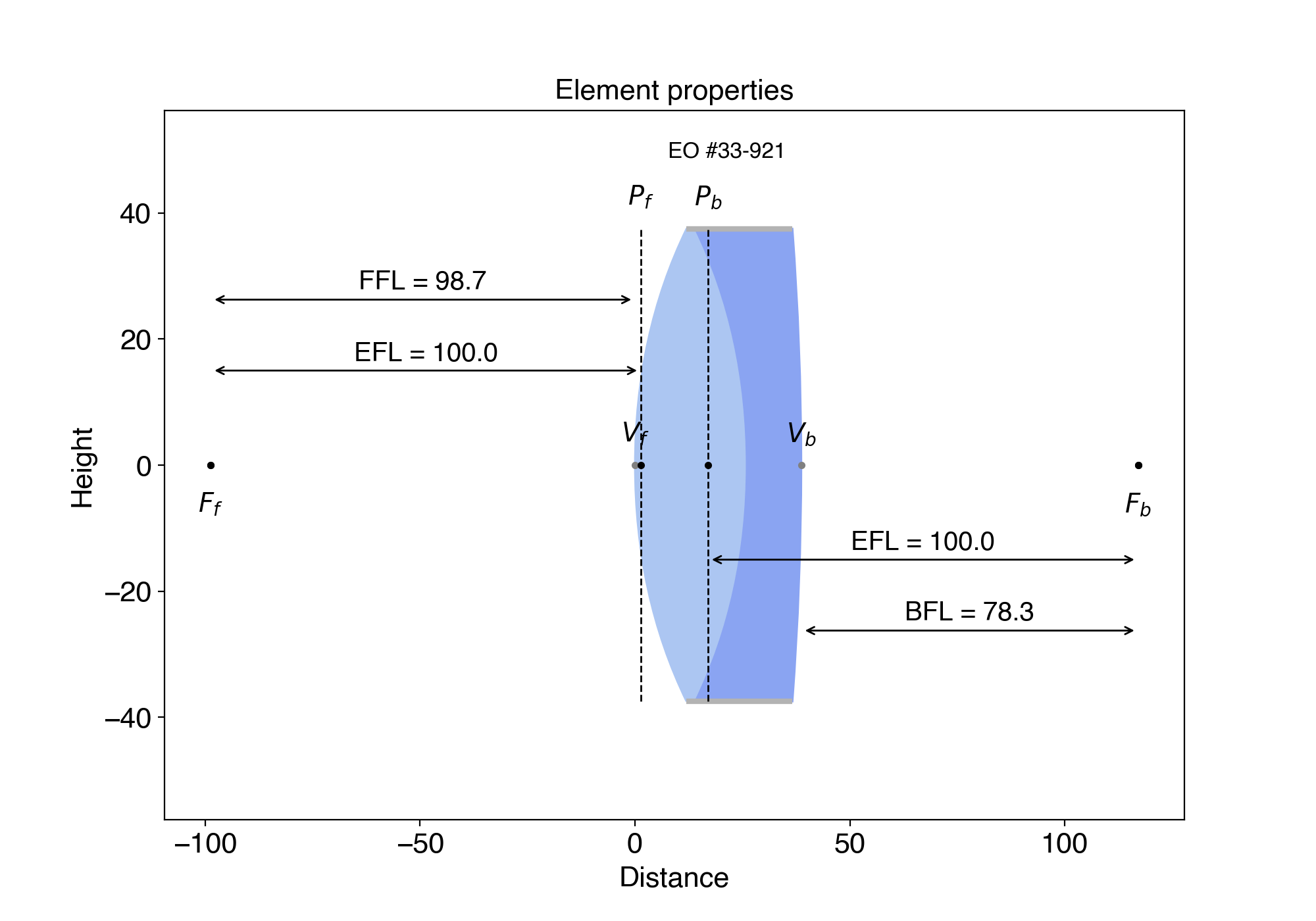
You can also call display() on an element to see the cardinal points, principal planes, BFL (back focal length, or the distance between the last interface and the focal point after the lens) and FFL (front focal length, or the distance between the focal point before the lens and the first interface). You can do it with any single Matrix element but also with MatrixGroup.
from raytracing import *

thorlabs.AC254_050_A().display()
eo.PN_33_921().display()
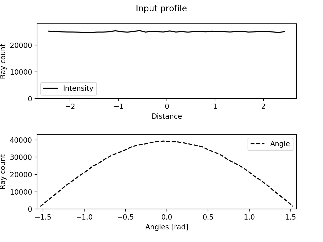
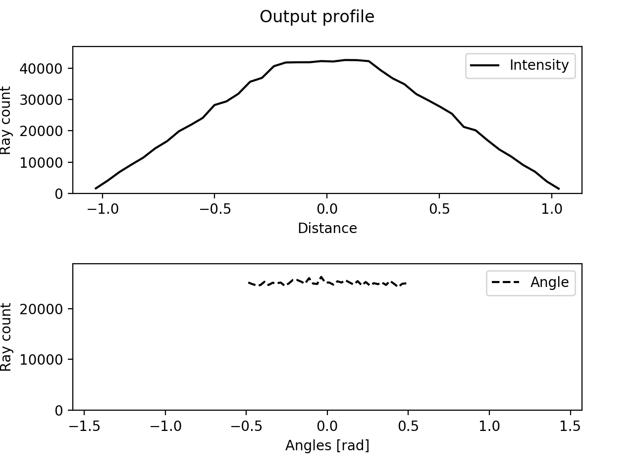
Finally, an addition as of 1.2.0 is the ability to obtain the intensity profile of a given source from the object plane at the exit plane of an OpticalPath. This is in fact really simple: by tracing a large number of rays, with the number of rays at y and θ being proportionnal to the intensity, one can obtain the intensity profile by plotting the histogram of rays reaching a given height at the image plane. Rays are small classes that return a Ray that satisfies the condition of the class. Currently, there is UniformRays,RandomUniformRays LambertianRays and RandomLambertianRays (a Lambertian distribution follows a cosθ distribution, it is a common diffuse surface source). They appear like iterators and can easily be used like this example script:
from raytracing import *
from numpy import *
import matplotlib.pyplot as plt

# Kohler illumination with these variables
fobj = 5
dObj = 5
f2 = 200
d2 = 50
f3 = 100
d3 = 50

# We build the path (i.e. not an Imaging path)
path = OpticalPath()
path.append(Space(d=f3))
path.append(Lens(f=f3, diameter=d3))
path.append(Space(d=f3))
path.append(Space(d=f2))
path.append(Lens(f=f2, diameter=d2))
path.append(Space(d=f2))
path.append(Space(d=fobj))
path.append(Lens(f=fobj, diameter=dObj))
path.append(Space(d=fobj))

# Obtaining the intensity profile
nRays = 1000000 # Increase for better resolution
inputRays = RandomLambertianRays(yMax=2.5, maxCount=nRays)
inputRays.display("Input profile")
outputRays = path.traceManyThrough(inputRays, progress=True)
# On macOS and Linux, you can do parallel computations.
# On Windows, who the hell knows? Maybe only on Windows 10 or Windows 7 32-bits, or whatever.
# outputRays = path.traceManyThroughInParallel(inputRays, progress=True, processes=8)
outputRays.display("Output profile")
and you will get the following ray histograms:
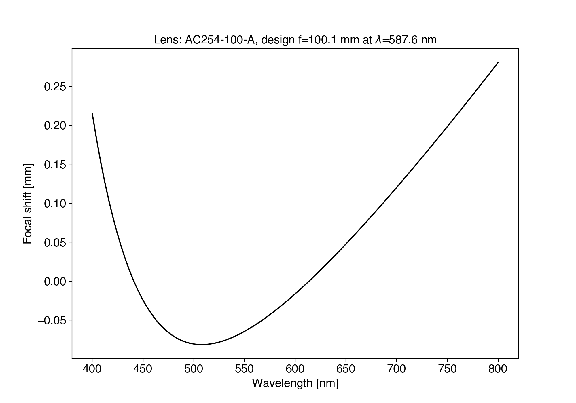
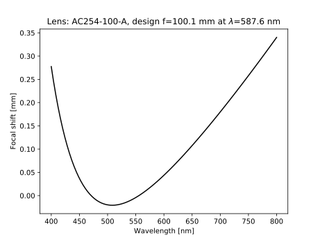
Finally, it is possible to obtain the chromatic aberrations for compound lenses (achromatic doublets from Thorlabs and Edmund optics, and singlet lens because the materials are known). The following command will give you the focal shift as a function of wavelength (as a graph or values):
from raytracing import *

thorlabs.AC254_100_A().showChromaticAberrations()
wavelengths, shifts = thorlabs.AC254_100_A().focalShifts()
Documentation
All the documentation is available online.
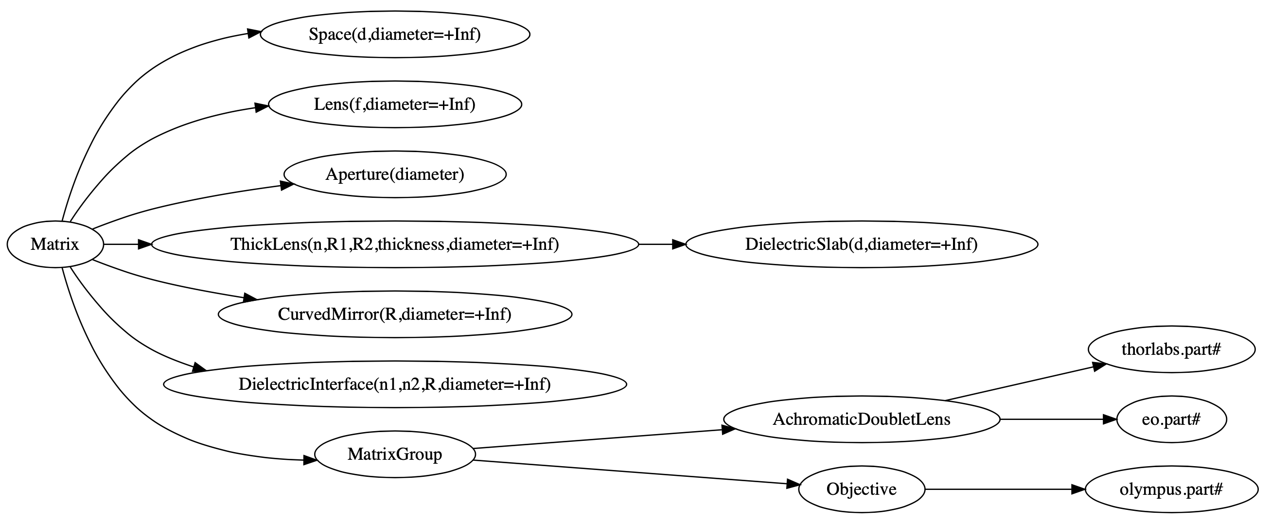
The class hierarchy for optical elements (with parameters and defaults) is:
You may obtain help by:
- Reading the documentation for the code (API reference).
- Core:
Ray: a ray for geometrical optics with a height and angle $y$ and $\theta$.Rays: ray distributions to ray trace an object through the optical system.UniformRays,RandomUniformRays,LambertianRaysandRandomLambertianRaysare currently available. See example above.
GaussianBeam: a gaussian laser beam with complex radius of curvature $q$.Matrix: any 2x2 matrix.MatrixGroup: treats a group of matrix as a unit (draws it as a unit too)ImagingPath: AMatrixGroupwith an object at the front for geometrical opticsLaserPath: AMatrixGroupwith a laser beam input at the front or a Resonator.
- Optical elements:
Aperture,Space,Lens,DielectricInterface,DielectricSlab,ThickLens - Specialty lenses: Defines a general achromat and objective lens
- Thorlabs lenses: Achromat doublet lenses from Thorlabs.
- Edmund Optics lenses: Achromat doublet lenses from Edmund Optics
- Olympus objectives: A few objectives from Olympus.
- Glasses: A few glasses used by Thorlabs to make achromatic doublets. They all have a single function
n(wavelength)that returns the index at that wavelength. All data obtained from http://refractiveindex.info. - Zemax ZMX file reader: to read text-based Zemax files of lenses.
- Core:
- typing (interactively):
help(Matrix),help(MatrixGroup)help(Ray),help(ImagingPath)to get the API, - look at the examples with
python -m raytracing - simply look at the code.
python
>>> help(Matrix)
Help on class Matrix in module raytracing.abcd:

class Matrix(builtins.object)
 |  Matrix(A, B, C, D, physicalLength=0, apertureDiameter=inf, label='')
 |
 |  A matrix and an optical element that can transform a ray or another
 |  matrix.
 |
 |  The general properties (A,B,C,D) are defined here. The operator "*" is
 |  overloaded to allow simple statements such as:
 |
 |  ray2 = M1 * ray
 |  or
 |  M3 = M2 * M1
 |
 |  The physical length is included in the matrix to allow simple management of
 |  the ray tracing. IF two matrices are multiplied, the resulting matrice
 |  will have a physical length that is the sum of both matrices.
 |
 |  In addition finite apertures are considered: if the apertureDiameter
 |  is not infinite (default), then the object is assumed to limit the
 |  ray height to plus or minus apertureDiameter/2 from the front edge to the back
 |  edge of the element.
 |
 |  Methods defined here:
 |
 |  __init__(self, A, B, C, D, physicalLength=0, apertureDiameter=inf, label='')
 |      Initialize self.  See help(type(self)) for accurate signature.
 |
 |  __mul__(self, rightSide)
 |      Operator overloading allowing easy to read matrix multiplication
 |
 |      For instance, with M1 = Matrix() and M2 = Matrix(), one can write
 |      M3 = M1*M2. With r = Ray(), one can apply the M1 transform to a ray
 |      with r = M1*r
 |
 |  __str__(self)
 |      String description that allows the use of print(Matrix())
 |
 |  backwardConjugate(self)
 |      With an image at the back edge of the element,
 |      where is the object ? Distance before the element by
 |      which a ray must travel to reach the conjugate plane at
 |      the back of the element. A positive distance means the
 |      object is "distance" in front of the element (or to the
 |      left, or before).
 |
 |      M2 = M1*Space(distance)
 |      # M2.isImaging == True
Examples
You can list several examples python -m raytracing -l:
All example code on your machine is found at: /somedirectory/on/your/machine
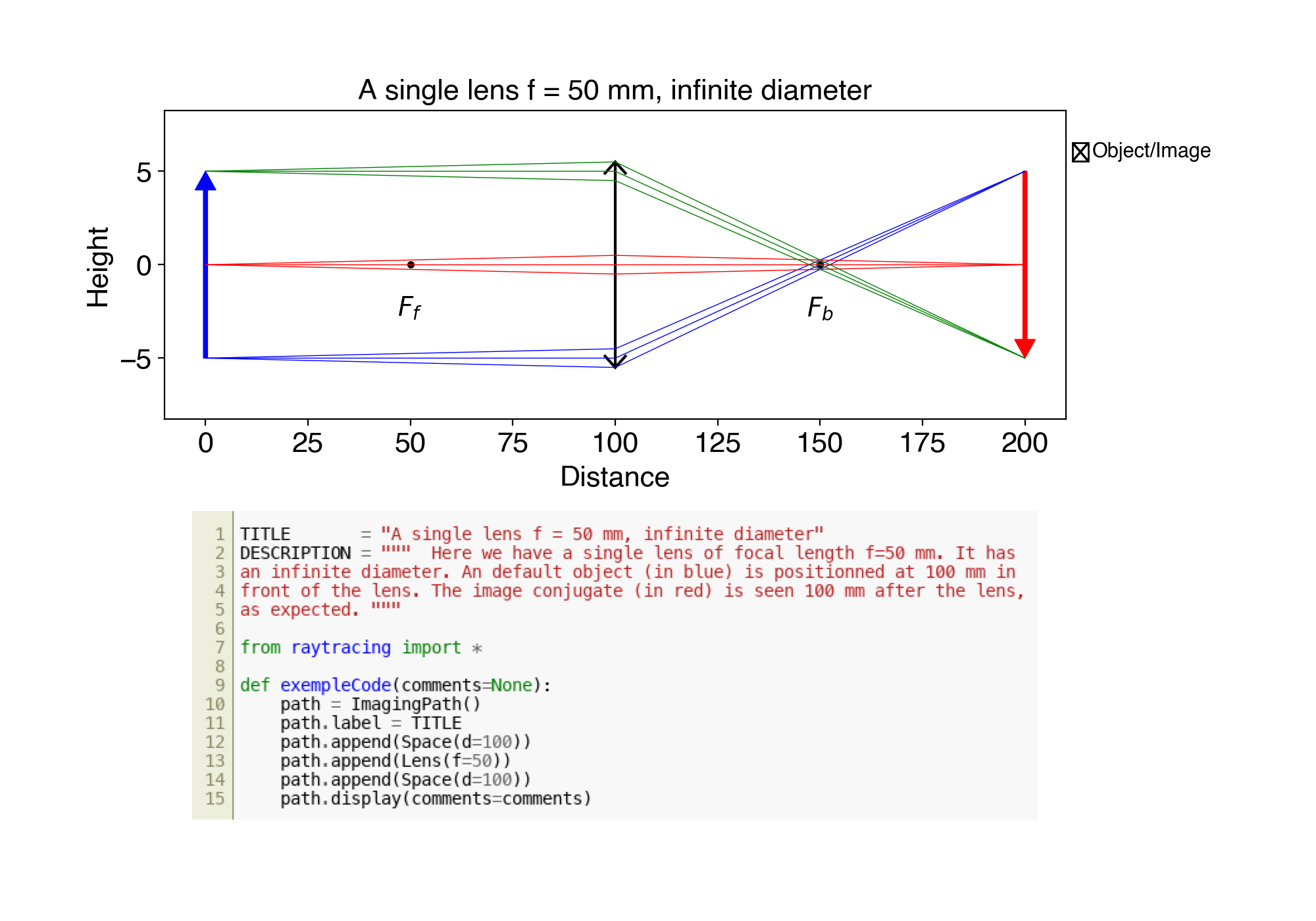
 1. ex01.py A single lens f = 50 mm, infinite diameter
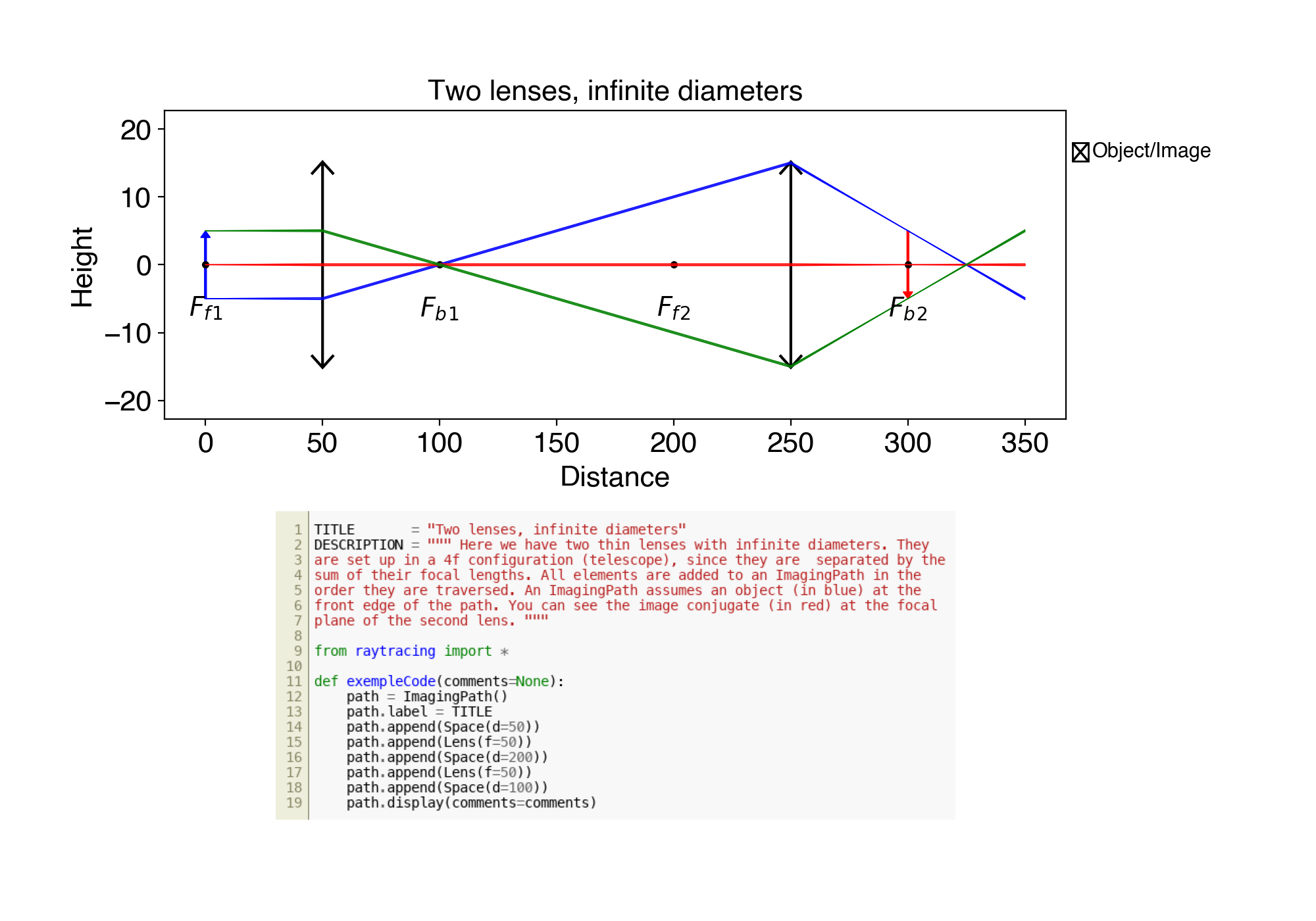
 2. ex02.py Two lenses, infinite diameters
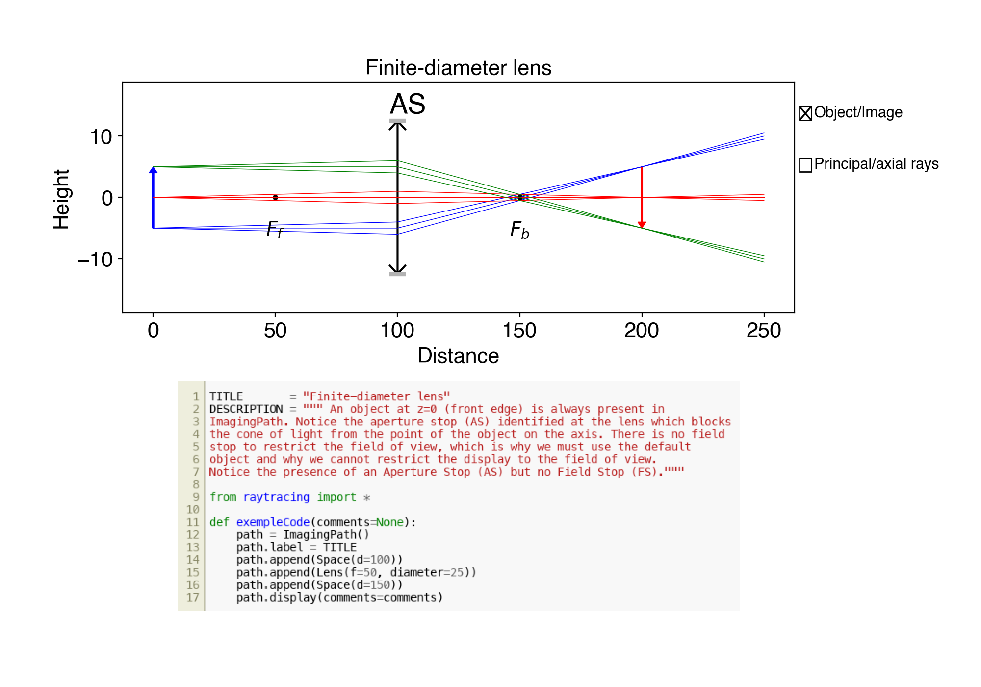
 3. ex03.py Finite-diameter lens
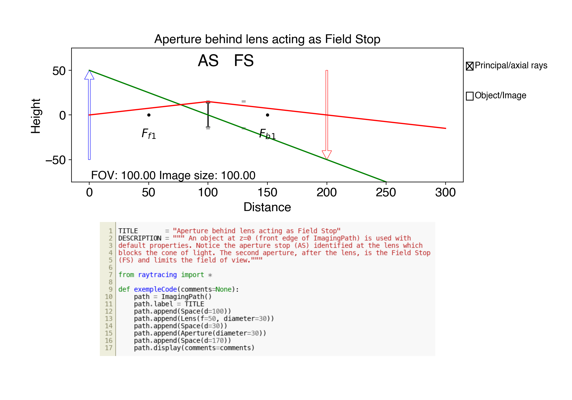
 4. ex04.py Aperture behind lens acting as Field Stop
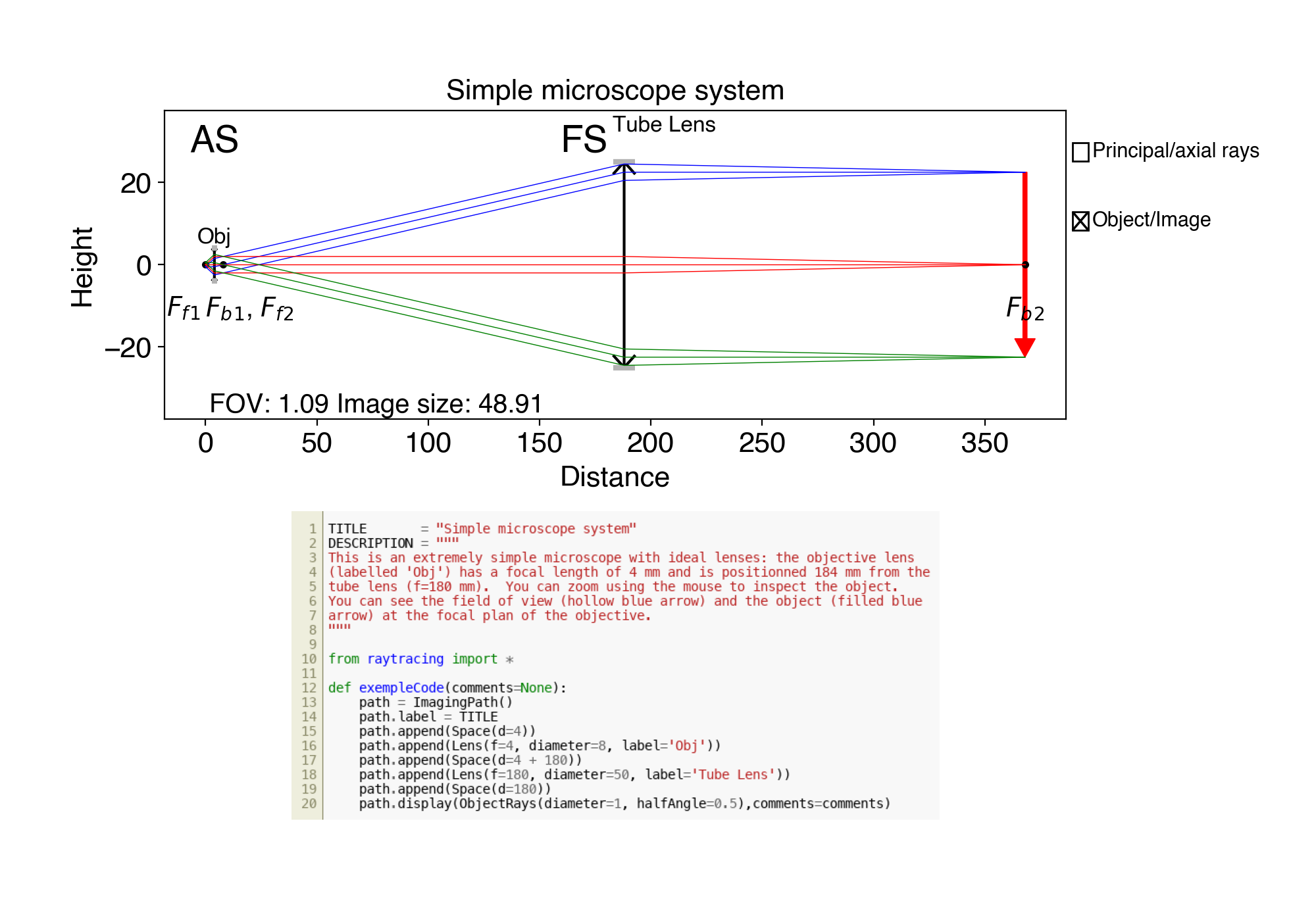
 5. ex05.py Simple microscope system
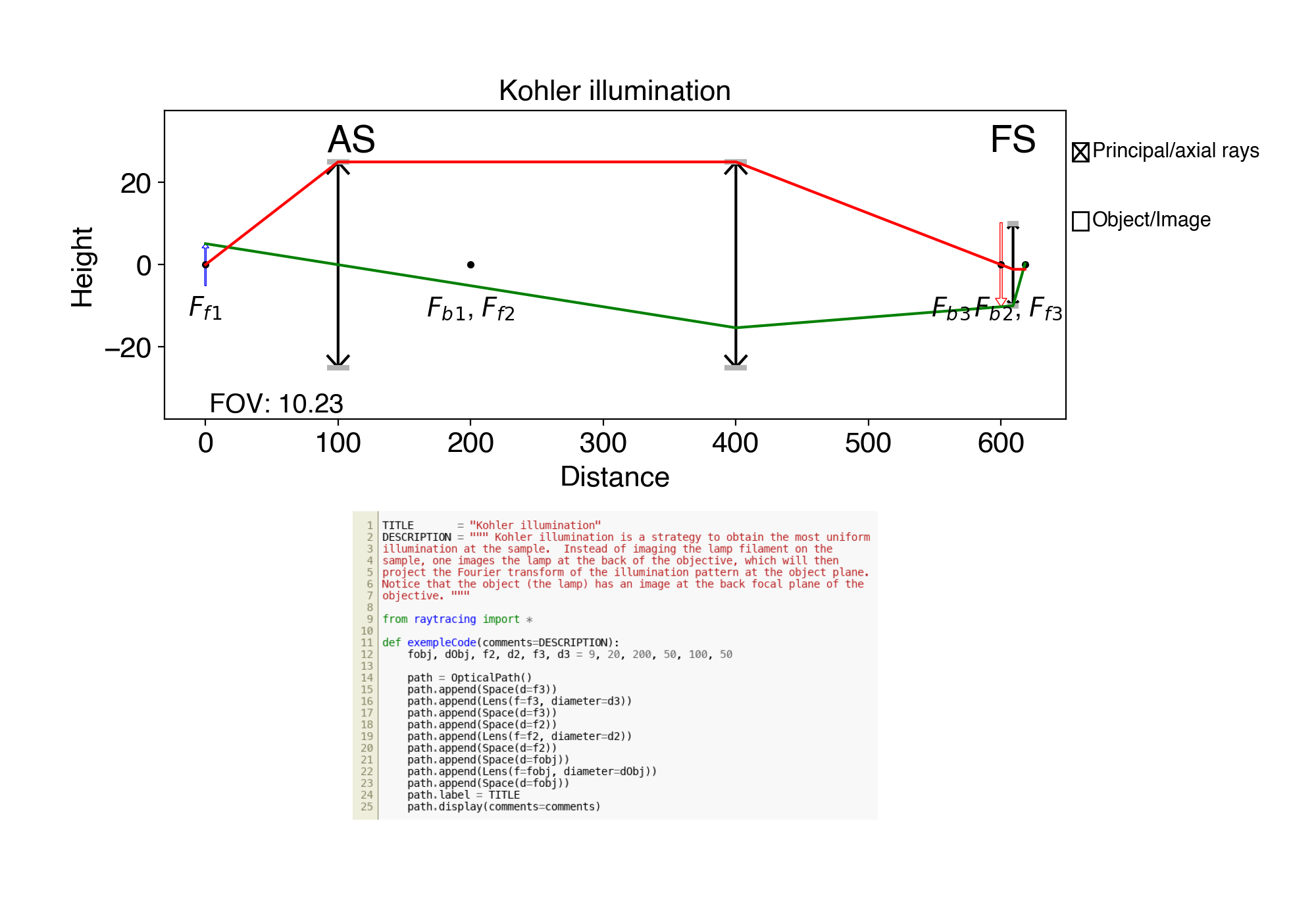
 6. ex06.py Kohler illumination
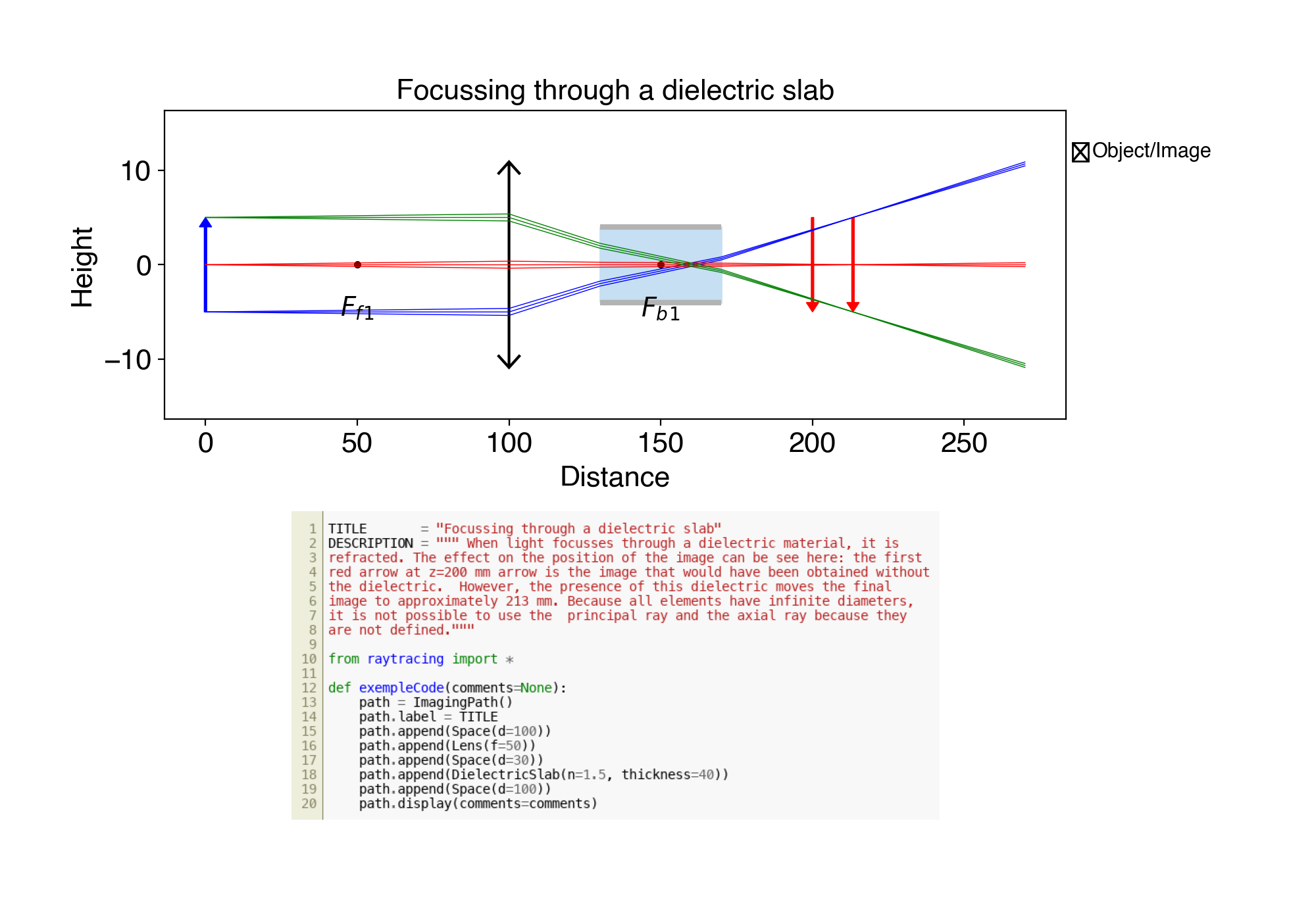
 7. ex07.py Focussing through a dielectric slab
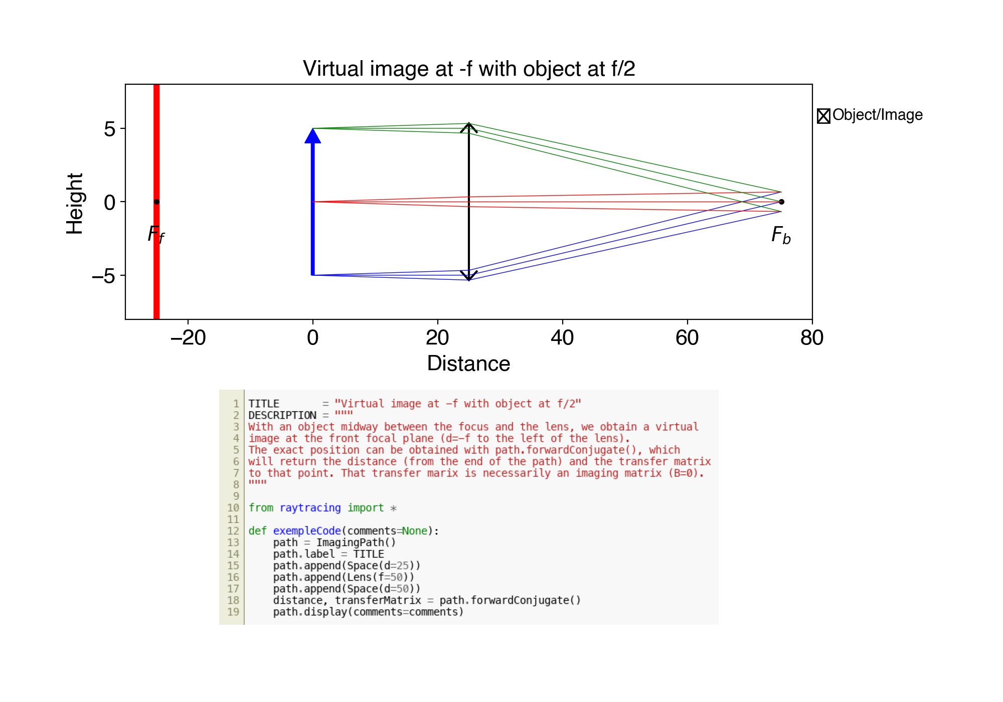
 8. ex08.py Virtual image at -f with object at f/2
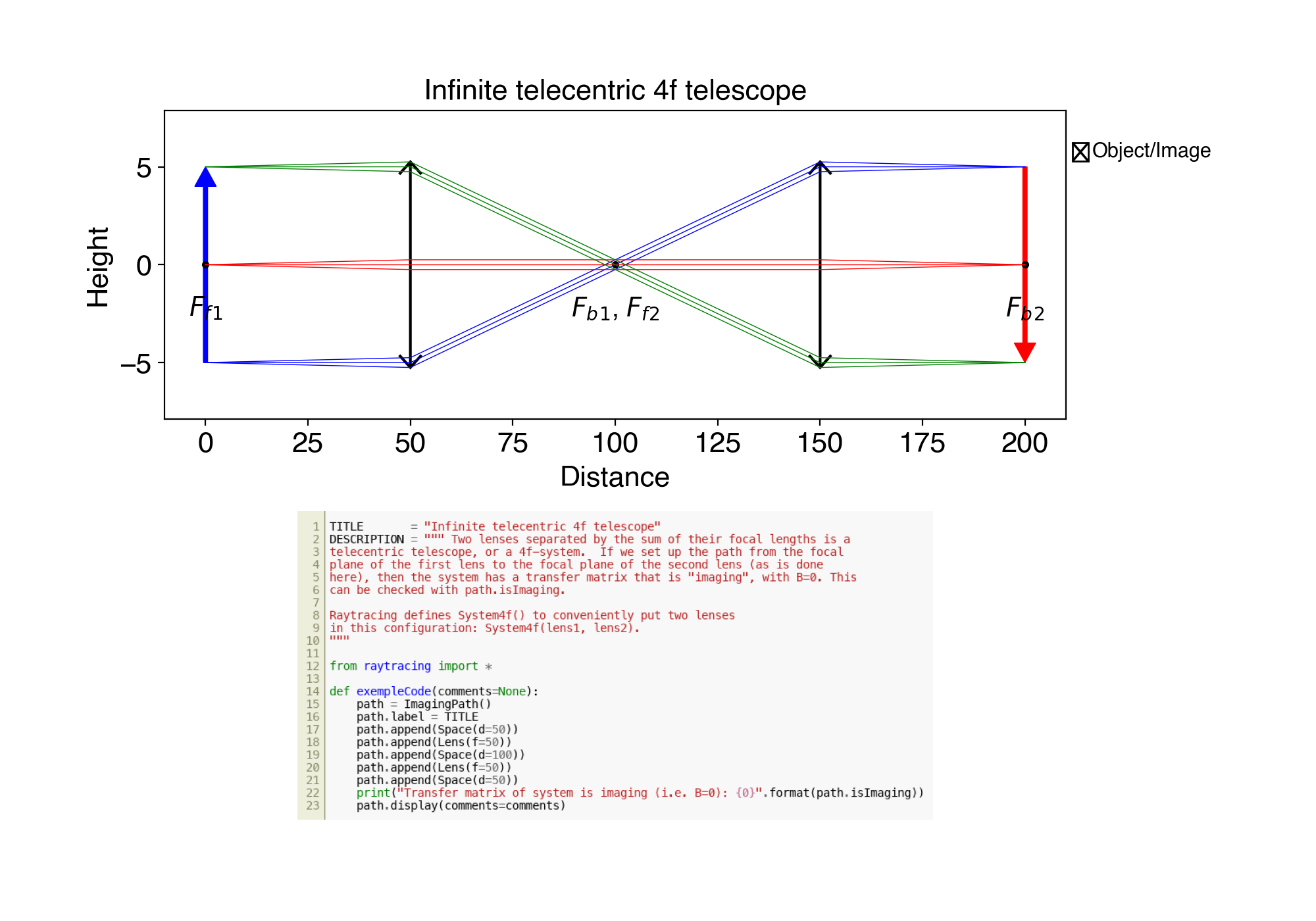
 9. ex09.py Infinite telecentric 4f telescope
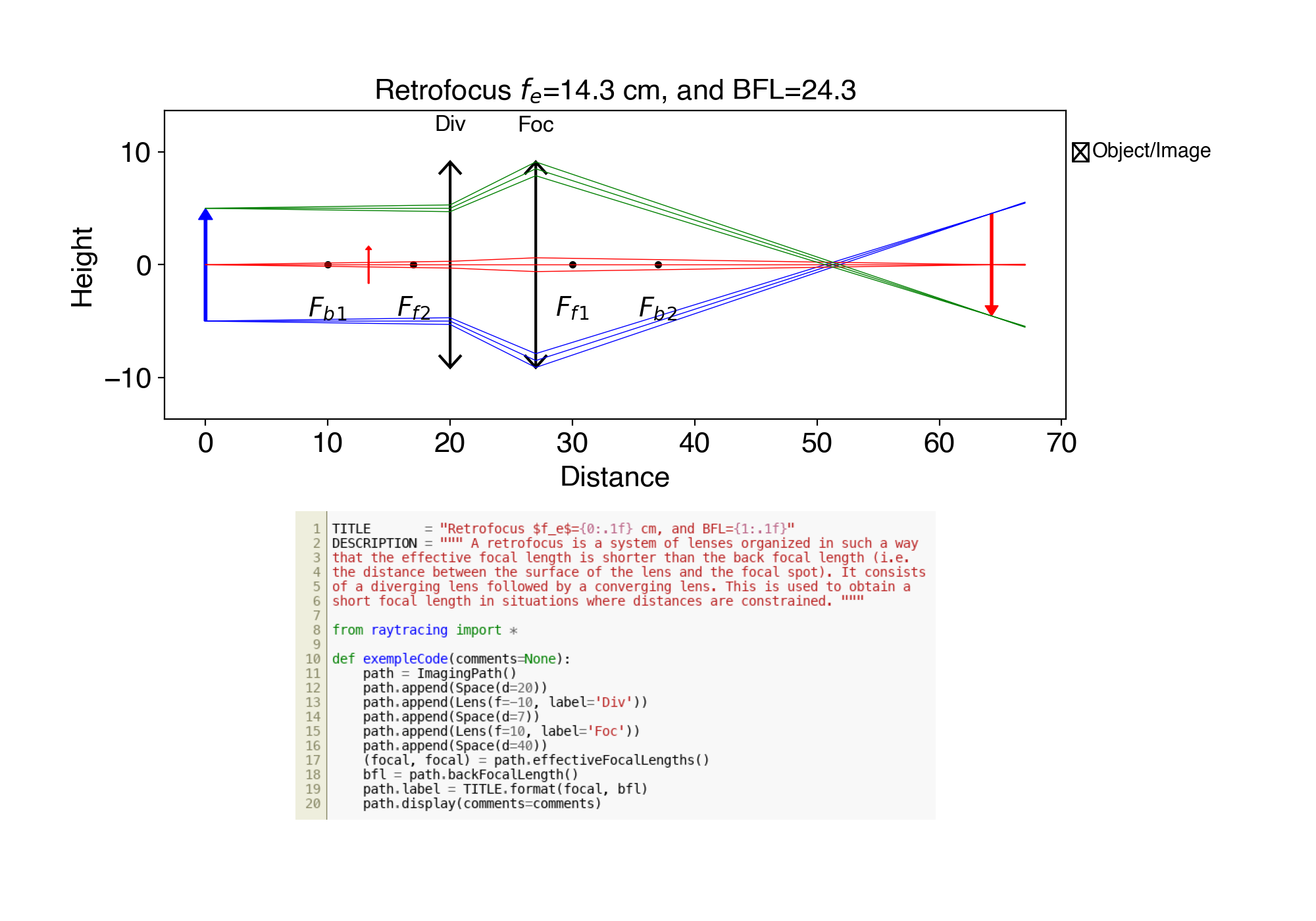
10. ex10.py Retrofocus $f_e$={0:.1f} cm, and BFL={1:.1f}
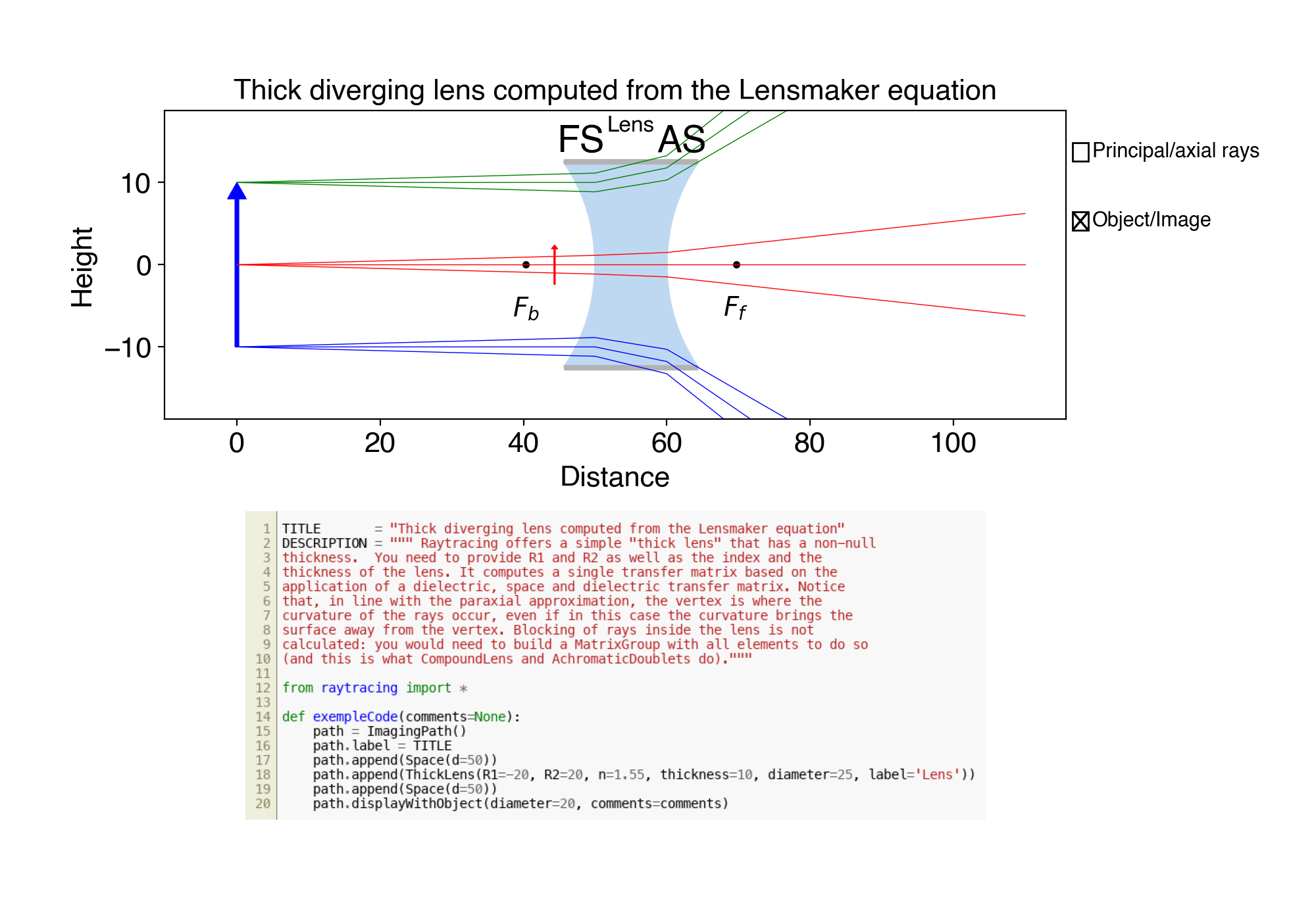
11. ex11.py Thick diverging lens computed from the Lensmaker equation
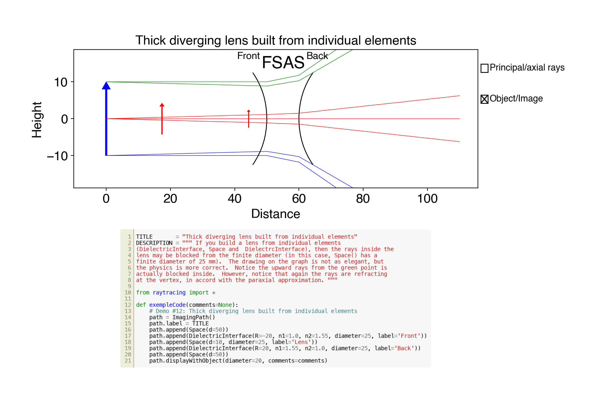
12. ex12.py Thick diverging lens built from individual elements
13. ex13.py Obtain the forward and backward conjugates
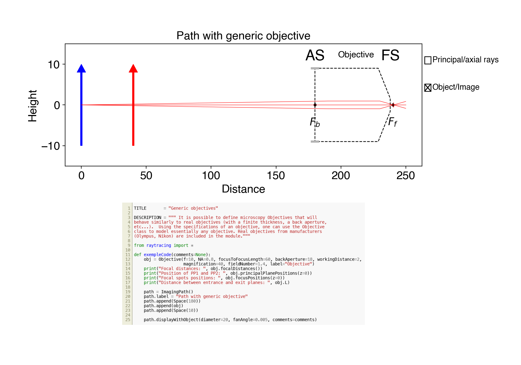
14. ex14.py Generic objectives
15. ex15.py Model Olympus objective LUMPlanFL40X
16. ex16.py Commercial doublets from Thorlabs and Edmund
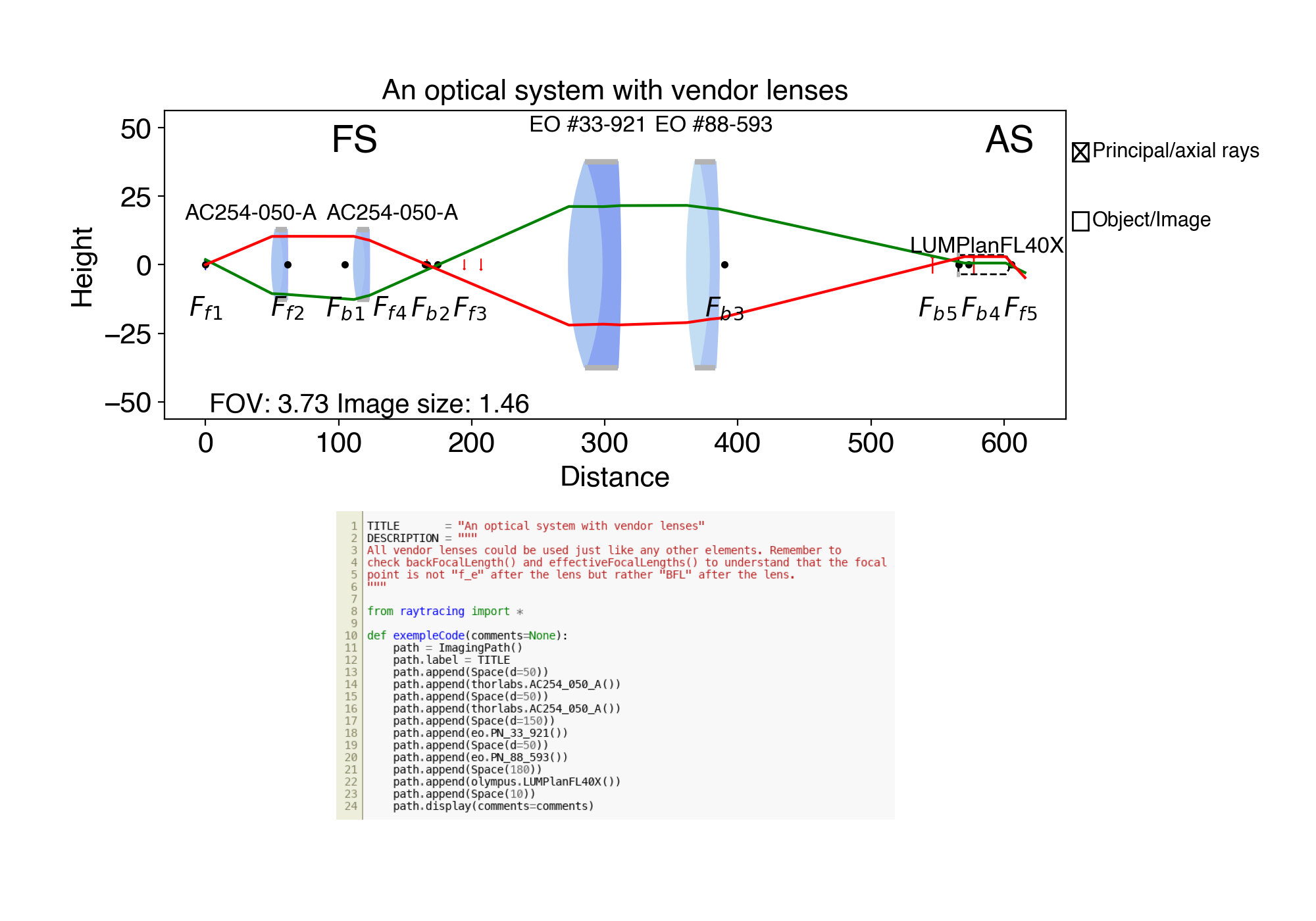
17. ex17.py An optical system with vendor lenses
18. ex18.py Laser beam and vendor lenses
19. ex19.py Cavity round trip and calculated laser modes
.... and more complete examples at /somedirectory/on/your/machine
You can run them all with python -m raytracing -e all (see them all below) to get a flavour of what is possible (note: in the US, it will give you a flavor of what is possible instead). Notice the command will tell you where the directory with all the tests is on your machine. You will find more complete examples in that examples directory, distributed with the module. For instance, illuminator.py to see a Kohler illuminator, and invariant.py to see an example of the role of lens diameters to determine the field of view.
GPU-accelerated ray tracing with OpenCL
As of version 1.4.0, the module supports GPU-accelerated batch ray tracing via OpenCL. When tracing large numbers of rays (100k–1M+) through an optical system, the GPU can provide 10–100x speedup over the pure-Python path.
Highlights
- Contiguous memory layout:
CompactRaysstores all ray data in a single numpy structured array (24 bytes per ray), ready for GPU transfer in one call. Individual rays are accessed through lightweightCompactRayviews that behave exactly like regularRayobjects. - On-device ABCD matrix multiplication: An OpenCL kernel runs one GPU workitem per ray, propagating it through all optical elements in sequence — including aperture blocking.
- Organized output: The flat GPU output buffer is wrapped by
CompactRaytraceandCompactRaytraces, giving convenient per-ray access to the full trace through the system without copying any data. - Optional dependency:
pyopenclis only imported when you calltraceManyOpenCL(). The rest of the module works without it.
Quick example
from raytracing import *
from raytracing.compact import CompactRays

path = ImagingPath()
path.append(Space(d=10))
path.append(Lens(f=50, diameter=25))
path.append(Space(d=100))
path.append(Lens(f=50, diameter=25))
path.append(Space(d=10))
group = MatrixGroup(path.transferMatrices())

rays = CompactRays(maxCount=1_000_000)
rays.fillWithRandomUniform(yMax=5)

# GPU path (requires pyopencl)
traces = group.traceManyOpenCL(rays)
traces.lastRays.display("Output profile (OpenCL)")
Known limitations
There are no known bugs in the actual calculations, but there are bugs or limitations in the display:
- It is not easy to put several labels on a graph without any overlap. We are still working on it.
- It is also not easy to figure out what "the right size" should be for an arrow head, the font, the position of a label, the size of the "ticks" on the aperture.
- Labelling focal points with appropriate secondary labels should be possible, maybe a superscript?
- The y-scale is not always set appropriately when the elements have infinite diameters: the rays will go beyond the element drawn on the figure.
Licence
This code is provided under the MIT License.
Project details
Release history Release notifications | RSS feed
Download files
Download the file for your platform. If you're not sure which to choose, learn more about installing packages.
Source Distribution
Built Distribution
Filter files by name, interpreter, ABI, and platform.
If you're not sure about the file name format, learn more about wheel file names.
Copy a direct link to the current filters
File details
Details for the file raytracing-1.4.7.tar.gz.
File metadata
- Download URL: raytracing-1.4.7.tar.gz
- Upload date:
- Size: 9.0 MB
- Tags: Source
- Uploaded using Trusted Publishing? No
- Uploaded via: twine/6.2.0 CPython/3.11.15
File hashes
| Algorithm | Hash digest | |
|---|---|---|
| SHA256 |
8928b0b976e0a921012595c571c630f2fbafdfa2e8c6c9d0517245faf6d6b5b1
|
|
| MD5 |
34d896d734c0abd38ce18180c5345eed
|
|
| BLAKE2b-256 |
a2d331dfa560f403f67a73b13a4652f25a1e5cad72d7aa6053f7c6b33917eace
|
File details
Details for the file raytracing-1.4.7-py3-none-any.whl.
File metadata
- Download URL: raytracing-1.4.7-py3-none-any.whl
- Upload date:
- Size: 230.4 kB
- Tags: Python 3
- Uploaded using Trusted Publishing? No
- Uploaded via: twine/6.2.0 CPython/3.11.15
File hashes
| Algorithm | Hash digest | |
|---|---|---|
| SHA256 |
7326406d9364ab19cb3a4e0df6fb2bf3205656d5bea62314a9ebee9d08115c19
|
|
| MD5 |
854bdb8e5433a4b772b23567be7aa760
|
|
| BLAKE2b-256 |
b659e7f760e6fa31075cf1067ad5359bb7a6b24e201bd7c5550162292f0b9eb8
|


