Functional enrichment terms aggregator.

Project description
restring
Easy to use functional enrichment terms retriever and aggregator, designed for the wet biology researcher
Overview
restring works on user-supplied differentially expressed (DE) genes list, and automatically pulls and aggregates functional enrichment data from STRING.
It returns, in table-friendly format, aggregated results from analyses of multiple comparisons.
Results can readily be visualized via highly customizable heat/clustermaps and bubble plots to produce beautiful publication-grade pics. Plus, it's got a GUI!
What KEGG pathway was found in which comparisons? What pvalues? What DE genes annotated in that pathway were shared in those comparisons? How can I simultaneously show results for all my experimental groups, for all terms, all at once? This can all be managed by restring.
Check it out! We have a paper out in Scientific Reports, with detailed step-by-step installation and usage protocols, and real use cases implemented and discussed:
reString: an open-source Python software to perform automatic functional enrichment retrieval, results aggregation and data visualization
Stefano Manzini, Marco Busnelli, Alice Colombo, Franchi Elsa, Grossano Pasquale, Giulia Chiesa
PMID: 34873191 PMCID: PMC8648753 DOI: 10.1038/s41598-021-02528-0


Table of contents
-
restring as a Python module
Use case
Modern high-throughput -omic approaches generate huge lists of differentially expressed (DE) genes/proteins, which can in turn be used for functional enrichment studies. Manualy reviewing a large number of such analyses is time consuming, especially for experimental designs with more than a few groups. Let's consider this experimental setup:
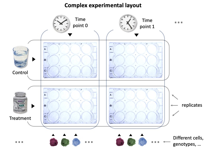
This represents a fairly common experimental design, but manually inspecting functional enrichment results for such all possible combinations would require substantial effort. Let's take a look at how we can tackle this issue with restring.
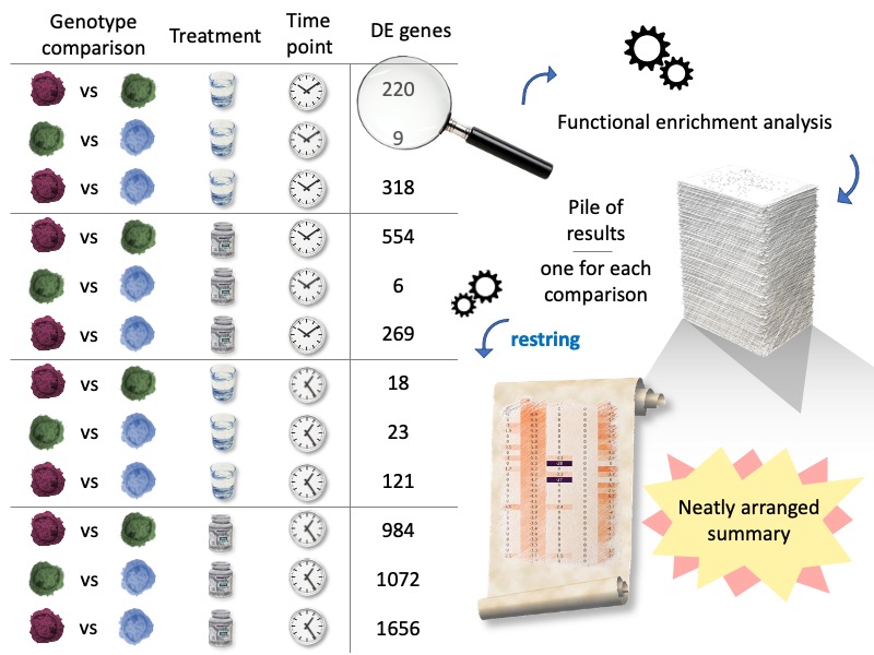
Our sample experimental setup has two treatments, given at two time points to three different sample types. Let's assume those samples are cells of different genotypes, and we'd like to mainly investigate genotype comparisons. After quantifying gene expression by RNAseq, we have DE genes for every comparison. As in many experimental pipelines, each list of DE genes is investigated with functional enrichment tools, such as String. But every comparison generates one or more tables. restring makes it easy to generate summary reports from all of them, automatically.
Installation
reString is a Python application, and requires Python to run. Please refer to Python's official page for installation: https://www.python.org/.
Once you have Python up and running, installing reString is as simple as opening up a terminal window and typing:
pip install restring
Here's what the installation process looks like in the Mac:
(restest) cln-169-032-dhcp:~ manz$ pip install restring
Collecting restring
  Downloading https://files.pythonhosted.org/packages/58/4c/03f7f06a15619bd8b53ada077a2e4f9d7cd187d9e9857ab57b3239963744/restring-0.1.16.tar.gz (1.2MB)
    100% |████████████████████████████████| 1.2MB 437kB/s
Requirement already satisfied: matplotlib in /Applications/Anaconda3/anaconda/lib/python3.4/site-packages (from restring)
Requirement already satisfied: seaborn in /Applications/Anaconda3/anaconda/lib/python3.4/site-packages (from restring)
Requirement already satisfied: pandas in /Applications/Anaconda3/anaconda/lib/python3.4/site-packages (from restring)
Requirement already satisfied: requests in /Applications/Anaconda3/anaconda/lib/python3.4/site-packages (from restring)
Requirement already satisfied: numpy>=1.6 in /Applications/Anaconda3/anaconda/lib/python3.4/site-packages (from matplotlib->restring)
Requirement already satisfied: python-dateutil in /Applications/Anaconda3/anaconda/lib/python3.4/site-packages (from matplotlib->restring)
Requirement already satisfied: pytz in /Applications/Anaconda3/anaconda/lib/python3.4/site-packages (from matplotlib->restring)
Requirement already satisfied: cycler in /Applications/Anaconda3/anaconda/lib/python3.4/site-packages (from matplotlib->restring)
Requirement already satisfied: pyparsing!=2.0.4,>=1.5.6 in /Applications/Anaconda3/anaconda/lib/python3.4/site-packages (from matplotlib->restring)
Requirement already satisfied: six>=1.5 in /Applications/Anaconda3/anaconda/lib/python3.4/site-packages (from python-dateutil->matplotlib->restring)
Building wheels for collected packages: restring
  Running setup.py bdist_wheel for restring ... done
  Stored in directory: /Users/manz/Library/Caches/pip/wheels/25/67/13/73711665f987ae891784bef729f350429599d2e3cda015a37a
Successfully built restring
Installing collected packages: restring
Successfully installed restring-0.1.16
(restest) cln-169-032-dhcp:~ manz$
To run restring, simply open a terminal and type:
restring-gui
This will launch reString in its GUI form. On Windows systems, the first time the antivirus might want to check restring-gui.exe, but the application should launch without issues once it realizes there are no threats.
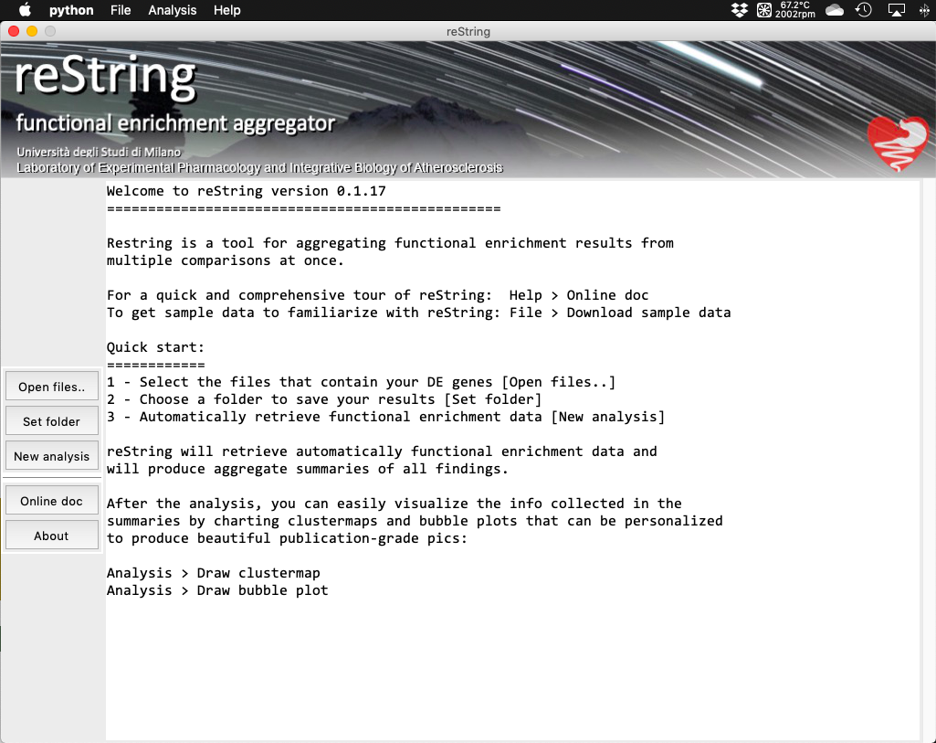
This is what it looks like in MacOS:
Installation in depth
Here are step-by-step instructions on how to install reString on specific platforms in the form of YouTube videos.
In each video description, the commands that should be inputted in the terminal to perfect the installation process are handily summarized. This covers both checking/installing Python, eventual missing dependencies and restring itself.
Installation troubleshooting
If you experience hiccups during the installation, maybe we got you covered:
- If you get
SyntaxErrorafter trying to runrestring:
make sure you are using Python 3.x and not Python 2.x.
Python 2.x is obsolete and discontinued. Many systems still support both, in this case you use python and pip for Python 2.x and python3 and pip3 or Python 3.x. In this case, use pip3 to install restring.
- If you get
SyntaxErrorand you are sure you're running Python 3.x:
then you're running a version prior to 3.6. Update it.
- If you get errors launching reString by typing
restring-gui:
To the exception of MacOS, we noticed that the installation script is not placed in the Path/PATH environment variable (that is: even if the script is in your computer, your computer doesn't know where to pull it from when you type it).
If this happens, you have two alternatives:
alternative a) start restring by typing
python -c "import restring; restring.restring_gui()"
or
python3 -c "import restring; restring.restring_gui()".
Use the first command if python is Python 3.x in your system, use python3 if in your system the version 2.x is called instead.
These commands are guaranteed to work from within any folder the terminal is in;
alternative b) permanently teach your system where the launch script lies. You will know the location from the installation log (refer to the YouTube videos). In GNU/linux systems, it's far easier to google for something like "how to permanently add a folder to PATH in YOUR_DISTRO_HERE". In Windows, follow the instructions of the YouTube installation guide. When done, you will be able to launch restring by just typing:
restring-gui
- If you get weird errors:
Get in touch with us: report a bug.
Procedure
restring can be used via its graphical user interface (recommended). A full protocol, with sample data and examples, is detailed below.
Alternatively, it can be imported as a Python module. This hands-on procedure is detailed at the end of this document.
restring GUI
1 | Prepping the files
All restring requires is a gene list of choice per experimental condition. This gene list needs to be in tabular form, arranged like this sample data. This is very easily managed with any spreadsheet editor, such as Microsoft's Excel or Libre Office's Calc.
2 | Set input files and output path
In the menu, choose File > Open..., or hit the Open files.. button.
Tip: put all input files you want to process together in one or more analyses in the same folder. Input files can be individually selected from any one folder, but each time input files are added, the input files list is reset.
Then, choose an existing directory where all putput files will be placed: choose File > Set output folder or hit Set folder button (Choose a different output folder each time the analysis parameters are varied, see section 5).
3 | Running the analysis with default settings
In the menu, choose Analysis > New analysis, or hit the New analysis button.
restring will look for genes in the files you have specified, interrogate STRING to get functional enrichment data back (these tables, looking exactly the same to the ones you would manually retrieve, will be saved into subfolders of the output folder), then write aggregated results and summaries.
These are found in the specified output directory, and take the form of results- or summary-type tables, in .tsv (tab separated values) format, that can be opened out-of-the-box by Excel or Calc. Let's take a look at the anatomy of these tables.
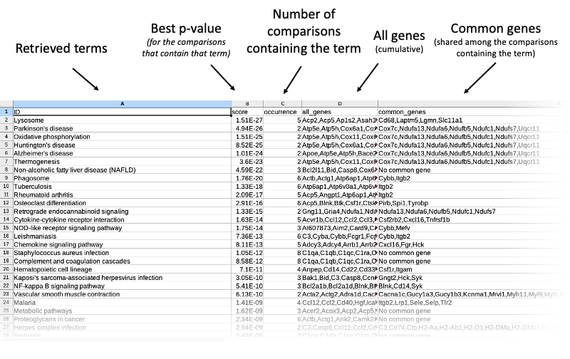
Results tables
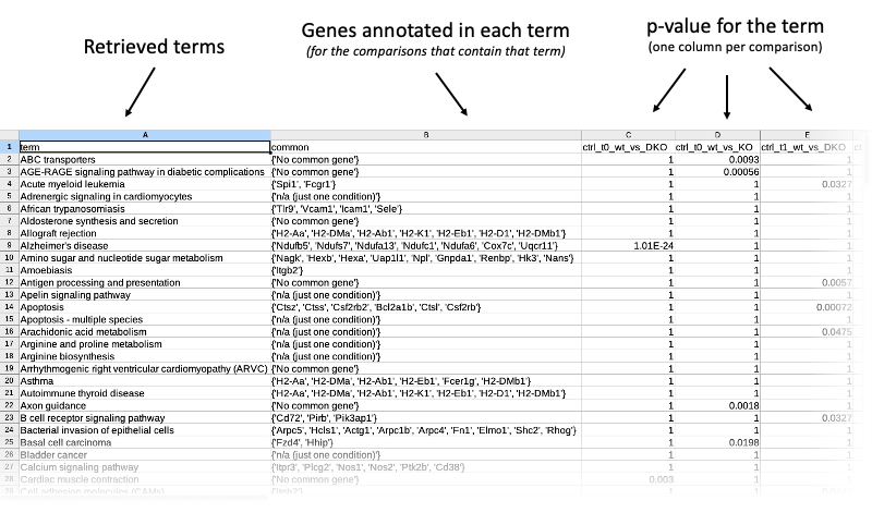
The table contains all terms cumulatively retrieved from all comparisons (each one of the inpt files containing the genes of interest between any two experimental conditions). For every term, common genes (if any) are listed. These common genes only include comparisons where the term actually shows up. If the term just appears in exactly one comparison, this is explicitly stated: n/a (just one condition). P-values are the ones retrieved from the STRING tables (the lower, the better). Missing p-values are represented with 1 (that is, in that specific comparison the term is 100% likely not enriched).
Summary tables
These can be useful to find the most interesting terms across all comparisons: better p-value, presence in most/selected comparisons), as well as finding the most recurring DE genes for each term.
4 | Visualizing the results
Clustermap
restring makes it easy to inspect the results by visualizing results-type tables as clustermaps.
In the menu, choose Analysis > Draw clustermap to open the Draw clustermap window:
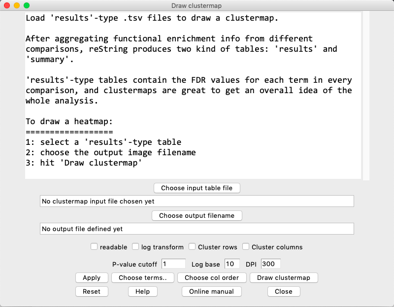
Clustermap Options
readable: if flagged, the output clustermap will be drawn as tall as required to fully display all the terms contained in it. Be warned that this might get very tall, depending on the number of terms.
log transform: if flagged, the p-values are minus log-transformed with the specified base: -log(number, base chosen). Hit Apply to apply.
cluster rows: if flagged, the rows are clustered (by distance) as per Scipy defaults. The column order is overridden.
cluster columns: if flagged, the columns are clustered (by distance) as per Scipy defaults.
P-value cutoff: For each term (row), if all values are higher than the specified threshold, the term is not included in the clustermap. For log-transformed heatmaps, for each term (row), if all values are lower than the specified threshold, the term is not included in the clustermap.
Insert a new value and hit Apply to see how many terms are retained/discarded by the new threshold.
Note that the default value of 1 will include all terms of a non-transformed table, as all terms are necessarily 1 or lower (moreover, there should automatically be at least a term per row that was significant, at P=0.05, in the files retrieved from STRING, otherwise the term would not appear in the table in the first place).
To set a new threshold, for instance at P=0.001, one should input 0.001, or 3 when log-transforming in base 10. Always hit Apply.
Log base: choose the base for the logarithm.
DPI: choose the output image resolution in DPI (dot per inch). The higher, the larger the image.
Apply: Applies the current settings to the table, and shows how the settings impact on the table.
Choose terms..: This button opens a dialog to choose the terms. An example:
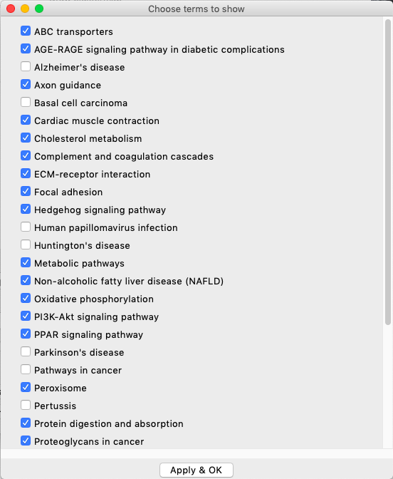
In this example, the results table contains terms that are irrelevant in the analysis being made. When loading a new table, all terms are automatically included, but the user chan choose to untick the terms that are unwanted. If a new P-value cutoff is applied, restring remembers the user choice even if some of the terms are now removed from the term list and are added back to the table at a later time.
Hit Apply & OK to apply the choice and close the window.
Choose col order: The user can reorder the column order by dragging the column names. Multiple adjacent columns can be selected and dragged together (this is ineffective if Cluster rows is flagged).
Hit OK to apply and close the window.
Draw clustermap: Draws, saves and opens the clustermap.
Reset: Reloads the input table and clears term selection.
Help: Opens a dialog that briefly outlines the procedure.
Online Manual: Opens the default browser at the clustermap help section.
Close: Closes the window.
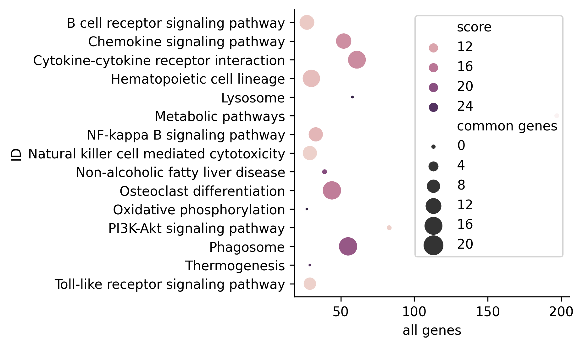
Bubble plot
restring makes it easy to inspect the results by visualizing summary-type tables as bubble plots.
In the menu, choose Analysis > Draw bubble plot to open the Draw bubble plot window:
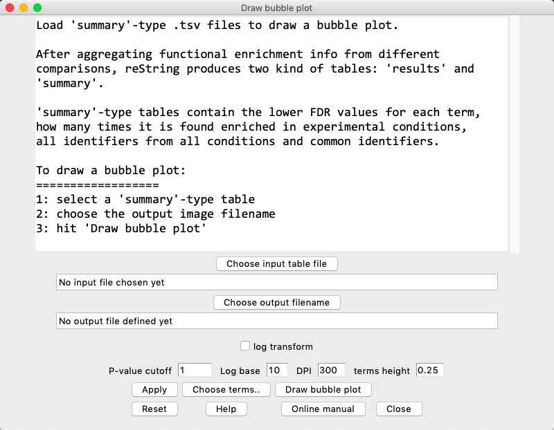
The bubble plot emphasizes the information gathered in summary-type tables, drawing, for each selected term, a bubble whose color and size reflect the FDR (color) and number of genes shared between all experimental conditions for each term (size). Here is an example:
Bubble plot options
log transform: if flagged, the p-values are minus log-transformed with the specified base: -log(number, base chosen). Hit Apply to apply.
P-value cutoff: For each term (row), if all values are higher than the specified threshold, the term is not included in the clustermap. For log-transformed heatmaps, for each term (row), if all values are lower than the specified threshold, the term is not included in the clustermap.
Insert a new value and hit Apply to see how many terms are retained/discarded by the new threshold.
Note that the default value of 1 will include all terms of a non-transformed table, as all terms are necessarily 1 or lower (moreover, there should automatically be at least a term per row that was significant, at P=0.05, in the files retrieved from STRING, otherwise the term would not appear in the table in the first place).
To set a new threshold, for instance at P=0.001, one should input 0.001, or 3 when log-transforming in base 10. Always hit Apply.
Log base: choose the base for the logarithm.
DPI: choose the output image resolution in DPI (dot per inch). The higher, the larger the image.
terms height: differently from the heatmap, bubble plots are always drawn such as all terms that survived the FDR cutoff and User selection are always readable. This parameter specifies how much distant (vertically) each term should be drawn in the resulting bubble plot. Defaults to 0.25.
Apply: Applies the current settings to the table, and shows how the settings impact on the table.
Choose terms..: This button opens a dialog to choose the terms. An example:
In this example, the results table contains terms that are irrelevant in the analysis being made. When loading a new table, all terms are automatically included, but the user chan choose to untick the terms that are unwanted. If a new P-value cutoff is applied, restring remembers the user choice even if some of the terms are now removed from the term list and are added back to the table at a later time.
Hit Apply & OK to apply the choice and close the window.
Draw bubble plot: Draws, saves and opens the bubble plot.
Reset: Reloads the input table and clears term selection.
Help: Opens a dialog that briefly outlines the procedure.
Online Manual: Opens the default browser at the bubble plot help section.
Close: Closes the window.
5 | Configuring the analysis.
Species
restring defaults to Mus musculus. To choose another species, choose Analysis > Set species to open the dialog:
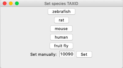
STRING accepts species in the form of taxonomy IDs. Hit the button of your species of choice or supply a custom TaxID and hit Set.
Head over to STRING's doc to know if your species is supported.
DE genes settings
restring accepts as gene lists input something like this sample data.
The input contains information of the gene name (we developed restring having the official gene name in mind as the preferred gene identifier, as that's always the case among researchers in our experience) and information about the direction of the change of expression with respect to experimental groups. This is the implied convention:
 gene ID  |  cond1  | cond2  | cond1_vs_cond2 |  log2FC |
 ---------|---------------------------------------------|
   gene1  |    143  |  748   |      0.191     |  -2.38  |
 ---------|---------------------------------------------|
   gene2  |    50   |   4    |      12.5      |   3.64  |
In this example, cond1 and cond2 are the two experimental condition where the abundance of the transcript has been estimated. Every RNAseq analysis contains at least the log2FC (base 2, log-transformed ratio of the expression values), that tells if the gene is upregulated or downregulated.
restring follows this convention:
UP is upregulated in cond1 versus cond2. That's the case of gene2. Log2FC is > 0.
DOWN is downregulated in cond1 versus cond2. That's the case of gene1. Log2FC is < 0.
restring does not actually care about the magnitude of Log2FC: that's from the pre-processing of the genes that the researcher is interested in.
Depending on how to treat the directionality information, there are four types of different analyses:
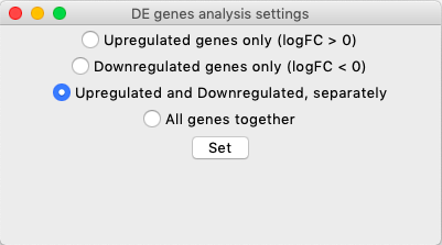
Upregulated genes only: Functional enrichment info is searched for upregulated genes only. Enrichment is performed on upregulated genes only (Arrange the input data so as "upregulated" in your experiment matches the implied convention).
Downregulated genes only: Functional enrichment info is searched for downregulated genes only. Enrichment is performed on downregulated genes only (Arrange the input data so as "downregulated" in your experiment matches the implied convention).
Upregulated and Downregulated, separately: This is the default option. For every comparison, both upregulated and downregulated genes are considered, but separately. This means that functional enrichment info is retrieved for upregulated and downregulated genes separately, but the terms are aggregated from both.
If a term shows up in both UP and DOWN gene lists, then the lowest P-value one is recorded.
All genes together: Functional enrichment info is searched for all genes together, and the resulting aggregation will reflect the functional enrichment analysis retrieved with all genes together (still supply a gene list that has a number, for each gene ID, in the second column. Just write any number.)
Tip: To avoid accumulating STRING files, consider setting a different output folder any time the analysis parameters are varied. Notwithstanding, restring clearly labels what enrichment files come from which gene lists: UP, DOWN or ALL are prepended to each table retrieved from STRING.
Set background
In the words of Szklarczyk et al. 2021's paper:
An increasing number of STRING users enter the database not with a single protein as their query, but with a set of proteins. [..] STRING will perform automated pathway-enrichment analysis on the user's input and list any pathways or functional subsystems that are observed more frequently than expected (using hypergeometric testing, against a statistical background of either the entire genome or a user-supplied background gene list).
By default, reString requests functional enrichment data against the statistical background of the entire genome. This is specified in the textual output during the anaysis:
Running the analysis against a statistical background of the entire genome (default).
Otherwise, it is possible to specify a background that will be applied to all input files, via Analysis > Custom background. You will be prompted to open a .csv, .tsv, .xls, .xlsx file that need to be a headerless, one-column file containing your custom background entries. Alternatively, you can place one entry per line in a .txt file. During the analysis, this will be specified as follows in the textual output:
Running the analysis against a statistical background of user-supplied terms.
Clear Background
To clear (empty) the custom background and revert to the default background (the entire genome), choose Analysis > Clear custom background. A message will confirm that the background has been cleared.
Choosing a specific STRING version
In the menu, choose Analysis > Choose STRING version to open the following dialog:
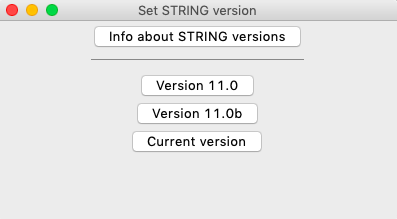
reString is compatible with the output produced from STRING API version 11.0 and above. To get info about past and current STRING releases, see here or hit Info about STRING versions in the window.
reString always defaults to the lastest release, but for compatibility purposes other versions (11.0b or 11.0) can be selected.
Need help?
Investigating an issue
Please let us know if you have any issue. From installation, to usage, to unforeseen application hiccups, there is a form to request assistance. Just hit New issue to start a new request. Files can be drag-and-dropped into the form as well, and your request can be previewed before being finalized.
To help up pin down the issue, please always include details about your machine setup (CPU, RAM, GPU, vendor) as well as your Python, OS and restring version. To further help investigating the matter, you should also include a procedure to allow us to replicate the issue in order to fix it (if possible, also include your input files).
If you've been encountering an issue, chances are that some other people have already stumbled over the same problem, and the answer might already be around in the Issues section.
Reporting a bug
Most of the time, restring communicates what it's doing by printing messages in the application window(s). In rare circumstances, errors are printed only to the terminal window (the one you've launched restring-gui from, and that's still around):
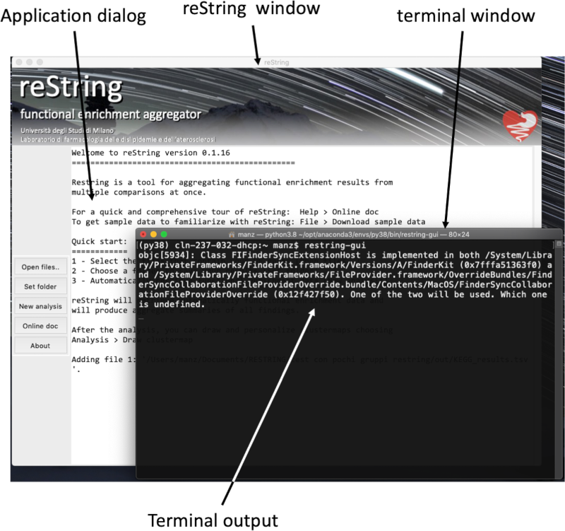
In addition to all information needed to investigate an issue (see above section), please include all terminal output (copy-and-paste the text, or drop a screenshot) in your bug report. Help us improve restring and report any bug here.
Requesting a new feature
If you feel like restring should be including some new awesome feature, please let us know! We are aimed at making restring richer and more user-friendly.
Known bugs
-
The repository of the ARM version of Raspberry Pi OS is sometimes having problems with keeping binaries up to date or working properly, and some of them might be required by
restring. If you experience installation troubles with that distribution, wait for the developers to get all packages up to date. -
When drawing a heatmap or a clustermap, if you load the wrong table type (e.g. a "results"-type table instead of a "summary"-type table,
restringwill complain but it will output some weird error to the terminal. Always keep an eye on what's going on in the terminal, as explained here. This will be fixed in the upcoming releases.
restring as a Python module
1 | Download required files from STRING
Head over to String, and analyze your gene/protein list. Please refer to the String documentation for help. After running the analysis, hit the 
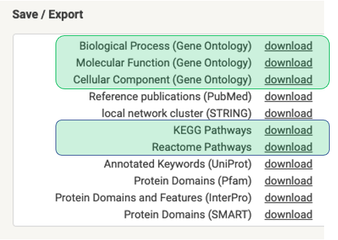
restring is designed to work with the results types highlighted in green. For each one of your experimental settings, create a folder with a name that will serve as a label for it. Here's how our sample data is arranged:
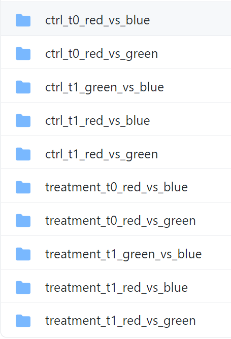
Not all comparisons resulted in a DE gene list that's long enough to generate functional enrichment results (see image above), thus a few comparisons (folders) are missing. When the DE gene list was sufficiently long to generate results for all analyses, this is what the folder content looks like (example of one folder):
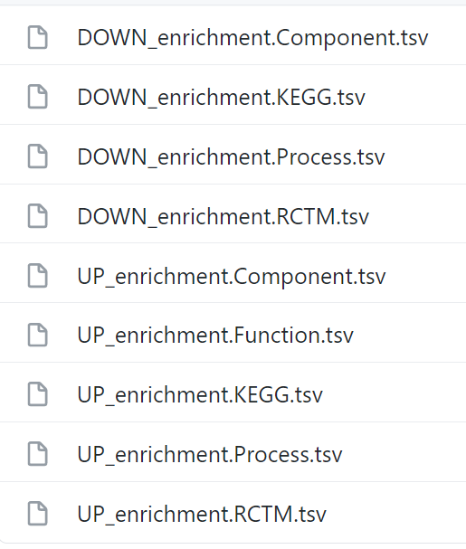
For each enrichment (KEGG, Component, Function, Process and RCTM), we fed String with DE genes that were either up- or downregulated with respect of one of the genotypes of the analysis. restring makes use of the UP and DOWN labels in the filenames to know what direction the analysis went (it's possible to aggregate UP and DOWN DE genes together).
It's OK to have folders that don't contain all files (if there were insufficient DE genes to produce some), like in the folder ctrl_t0_green_VS_ctrl_t0_blue_FC that you will find in your output directory after the analysis has finished.
2 | Aggregating the results
Once everything is set up, we can run restring to aggregate info from all the sparse results. The following example makes use of the String results that can be found in sample output.
import restring

dirs = restring.get_dirs()
print(dirs)
['ctrl_t0_green_VS_ctrl_t0_blue_FC',
 'ctrl_t0_green_VS_ctrl_t0_red_FC',
 'ctrl_t0_red_VS_ctrl_t0_blue_FC',
 'ctrl_t1_green_VS_ctrl_t1_blue_FC',
 'ctrl_t1_green_VS_ctrl_t1_red_FC',
 'ctrl_t1_red_VS_ctrl_t1_blue_FC',
 'treatment_t0_green_VS_treatment_t0_blue_FC',
 'treatment_t0_green_VS_treatment_t0_red_FC',
 'treatment_t0_red_VS_treatment_t0_blue_FC',
 'treatment_t1_green_VS_treatment_t1_blue_FC',
 'treatment_t1_green_VS_treatment_t1_red_FC',
 'treatment_t1_red_VS_treatment_t1_blue_FC']
get_dirs() returns a list of all folders within the current directory, to the excepion of folders beginning with __ or .. We can start aggregating results with default parameters (KEGG pathways for both UP and DOWN regulated genes).
db = restring.aggregate_results(dirs)
Start walking the directory structure.

Parameters
----------
folders: 12
kind=KEGG
directions=['UP', 'DOWN']

Processing directory: ctrl_t0_green_VS_ctrl_t0_blue_FC
Processing directory: ctrl_t0_green_VS_ctrl_t0_red_FC
	Processing file DOWN_enrichment.KEGG.tsv
	Processing file UP_enrichment.KEGG.tsv
Processing directory: ctrl_t0_red_VS_ctrl_t0_blue_FC
	Processing file DOWN_enrichment.KEGG.tsv
	Processing file UP_enrichment.KEGG.tsv
Processing directory: ctrl_t1_green_VS_ctrl_t1_blue_FC
Processing directory: ctrl_t1_green_VS_ctrl_t1_red_FC
	Processing file DOWN_enrichment.KEGG.tsv
	Processing file UP_enrichment.KEGG.tsv
Processing directory: ctrl_t1_red_VS_ctrl_t1_blue_FC
	Processing file DOWN_enrichment.KEGG.tsv
	Processing file UP_enrichment.KEGG.tsv
Processing directory: treatment_t0_green_VS_treatment_t0_blue_FC
Processing directory: treatment_t0_green_VS_treatment_t0_red_FC
	Processing file UP_enrichment.KEGG.tsv
Processing directory: treatment_t0_red_VS_treatment_t0_blue_FC
	Processing file DOWN_enrichment.KEGG.tsv
	Processing file UP_enrichment.KEGG.tsv
Processing directory: treatment_t1_green_VS_treatment_t1_blue_FC
	Processing file DOWN_enrichment.KEGG.tsv
	Processing file UP_enrichment.KEGG.tsv
Processing directory: treatment_t1_green_VS_treatment_t1_red_FC
	Processing file DOWN_enrichment.KEGG.tsv
	Processing file UP_enrichment.KEGG.tsv
Processing directory: treatment_t1_red_VS_treatment_t1_blue_FC
	Processing file DOWN_enrichment.KEGG.tsv
	Processing file UP_enrichment.KEGG.tsv

Processed 12 directories and 17 files.
Found a total of 165 KEGG elements.
Tip: you must start working in the same directory where you start restring, as it memorizes the starting directory at startup and would otherwise complain that it can longer locate the folders. tl;dr: don't play around with os.chdir(), get to the folder containing the output folders from the start.
Running aggregate_results() with other parameters is possible:
help(restring.aggregate_results)
# truncated output
    Walks the given <directories> list, and reads the String .tsv files of
    defined <kind>.

    Params:
    =======
    directories: <list> of directories where to look for String files

    kind:    <str> Defines the String filetype to process. Kinds defined in
             settings.file_types

    directions: <list> contaning the up- or down-regulated genes in a comparison.
             Info is retrieved from either UP and/or DOWN lists.
             * Prerequisite *: generating files form String with UP and/or DOWN regulated
             genes separately.

    verbose: <bool>; turns verbose mode on or off
The kind parameter is picked from the 5 supported String result tables:
print(restring.settings.file_types)
('Component', 'Function', 'KEGG', 'Process', 'RCTM')
To manipulate the aggregated results, it's convenient to put them into a table:
df = restring.tableize_aggregated(db)
This functions wraps the results into a handy pandas.DataFrame object, that can be saved as a table for further inspection:
df.to_csv("results.csv")
The table contains all terms cumulatively retrieved from all comparisons (directories/columns). For every term, common genes (if any) are listed. These common genes only include comparisons where the term actually shows up. If the term just appears in exactly one comparison, this is explicitly stated: n/a (just one condition). P-values are the ones retrieved from the String tables (the lower, the better). Missing p-values are represented with 1 (this can be set to anything str() accepts when calling tableize_aggregated() with the not_found parameter).
These 'aggregated' tables are useful for charting the results (see later). There's other info that can be extracted form aggregated results, in the form of a 'summary' table:
res = restring.summary(db)
res.to_csv("summary.csv")
These can be useful to find the most interesting terms across all comparisons: better p-value, presence in most/selected comparisons), as well as finding the most recurring DE genes for each term.
3 | Visualizing the results with a clustermap
'aggregated'-type tables can be readily transformed into beautiful clustermaps. This is simply done by passing either the df object previolsly created with tableize_aggregated(), or the file name of the table that was saved from that object to the draw_clustermap() function:
clus = restring.draw_clustermap("results.csv")
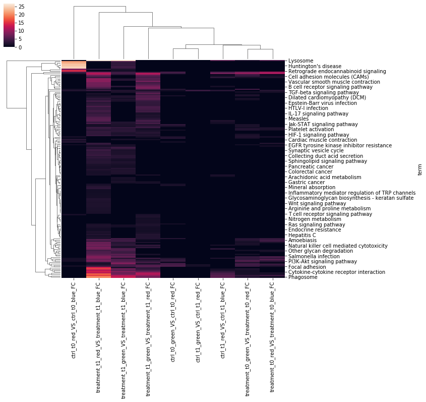
(The output may vary depending on your version of plotting libraries) Note that draw_clustermap() actually returns the seaborn.matrix.ClusterGrid object that it generates internally, this might come handy to retrieve the reordered (clustered) elements (more on that later).
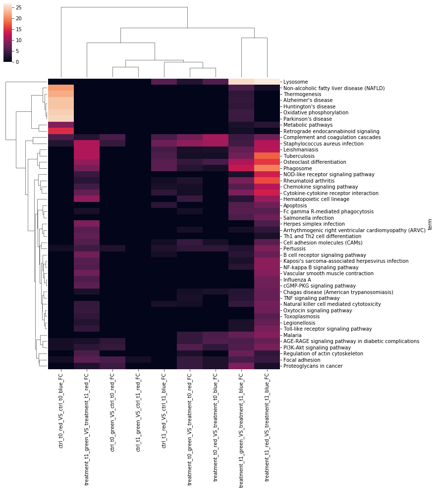
The drawing function is basically a wrapper for seaborn.clustermap(), of which retains all the flexible customization options, but allows for an immediate tweaking of the picture. For instance, we might just want to plot the highest-ranking terms and have all of them clearly written on a readable heatmap:
clus = restring.draw_clustermap("results.csv", pval_min=6, readable=True)
4 | Polishing up
More tweaking is possibile:
help(restring.draw_clustermap)
Help on function draw_clustermap in module restring.restring:

draw_clustermap(data, figsize=None, sort_values=None, log_transform=True, log_base=10,
                log_na=0, pval_min=None, custom_index=None, custom_cols=None,
		unwanted_terms=None, title=None, title_size=24, savefig=False,
		outfile_name='aggregated results.png', dpi=300, readable=False,
		return_table=False, **kwargs)

    Draws a clustermap of an 'aggregated'-type table.

    This functions expects this table layout (example):

    terms │ exp. cond 1 | exp. cond 2 | exp cond n ..
    ──────┼─────────────┼─────────────┼────────────..
    term 1│     0.01    |      1      |  0.00023
    ------┼-------------┼-------------┼------------..
    term 2│      1      |    0.05     |     1
    ------┼-------------┼-------------┼------------..
      ..  │     ..      |      ..     |     ..

    *terms* must be indices of the table. If present, 'common' column
    will be ignored.

    Params
    ------

    data      A <pandas.DataFrame object>, or a filename. If a filename is
              given, this will try to load the table as if it were produced
              by tableize_aggregated() and saved with pandas.DataFrame.to_csv()
              as a .csv file, with ',' as separator.

    sort_values   A <str> or <list> of <str>. Sorts the table accordingly. Please
              *also* set col_cluster=False (see below, seaborn.clustermap()
              additional parameters), otherwise columns will still be clustered.

    log_transform   If True, values will be log-transformed. Defaults to True.
              note: values are turned into -log values, thus p-value of 0.05
              gets transformed into 1.3 (with default parameters), as
              10^-1.3 ~ 0.05

    log_base  If log_transform, this base will be used as the logarithm base.
              Defaults to 10

    log_na    When unable to compute the logarithm, this value will be used
              instead. Defaults to 0 (10^0 == 1)

    pval_min  Trims values to the ones matching *at least* this p value. If
              log_transform with default values, this needs to be set accordingly
              For example, if at least p=0.01 is desired, then aim for
              pval_min=2 (10^-2 == 0.01)

    custom_cols   It is possible to pass a <list> of <str> to draw only specified
              columns of input table

    custom_index  It is possible to pass a <list> of <str> to draw only specified
              rows of input table

    unwanted_terms   If a <list> of <str> is supplied,

    readable  If set to False (default), the generated heatmap will be of reasonable
              size, possibly not showing all term descriptors. Setting readable=True
              will result into a heatmap where all descriptors are visible (this might
              result into a very tall heatmap)

    savefig   If True, a picture of the heatmap will be saved in the current directory.

    outfile_name  The file name of the picture saved.

    dpi       dpi resolution of saved picture. Defaults to 300.

    return_table   If set to True, it also returns the table that was manipulated
              internally to draw the heatmap (with all modifications applied).
              Returns: <seaborn.matrix.ClusterGrid>, <pandas.core.frame.DataFrame>

    **kwargs    The drawing is performed by seaborn.clustermap(). All additional
              keyword arguments are passed directly to it, so that the final picture
              can be precisely tuned. More at:
              https://seaborn.pydata.org/generated/seaborn.clustermap.html
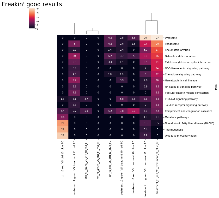
With a few brush strokes we can obtain the picture we're looking for. Example:
bad = [
    "Alzheimer's disease",
    "Huntington's disease",
    "Parkinson's disease",
    "Retrograde endocannabinoid signaling",
    "Staphylococcus aureus infection",
    "Tuberculosis",
    "Leishmaniasis",
    "Herpes simplex infection",
    "Kaposi's sarcoma-associated herpesvirus infection",
    "Proteoglycans in cancer",
    "Pertussis",
    "Malaria",
    "I'm not in the index"
]

clus = restring.draw_clustermap(
    "results.csv", pval_min=8, title="Freakin' good results", unwanted_terms=bad,
    sort_values="treatment_t1_wt_vs_DKO", row_cluster=False, annot=True,
)
Release history Release notifications | RSS feed


Download files
Download the file for your platform. If you're not sure which to choose, learn more about installing packages.
Source Distribution
File details
Details for the file restring-0.1.21.tar.gz.
File metadata
- Download URL: restring-0.1.21.tar.gz
- Upload date:
- Size: 1.4 MB
- Tags: Source
- Uploaded using Trusted Publishing? No
- Uploaded via: twine/4.0.2 CPython/3.10.10
File hashes
| Algorithm | Hash digest | |
|---|---|---|
| SHA256 |
a41c398a1c5a0b005f218f4eff211f00aa7e2d639204233bae49332b605ea76e
|
|
| MD5 |
bf98b937a70183cd3dbc39f6565b75a0
|
|
| BLAKE2b-256 |
4389f8fcb9451354582162b021ac7dc44848eb2feb860bd13c907a05732529dd
|


