Microbe-metabolite interactions through neural networks

Project description

rhapsody
Neural networks for estimating microbe-metabolite interactions through their co-occurence probabilities.
Installation
Rhapsody can be installed via pypi as follows
pip install rhapsody
If you are planning on using GPUs, be sure to pip install tensorflow-gpu.
Rhapsody can also be installed via conda as follows
conda install rhapsody -c conda-forge
Note that this option may not work in cluster environments, it maybe workwhile to pip install within a virtual environment. It is possible to pip install rhapsody within a conda environment, including qiime2 conda environments. However, pip and conda are known to have compatibility issues, so proceed with caution.
Getting started
To get started you can run a quick example as follows. This will learn microbe-metabolite vectors (mmvec) which can be used to estimate microbe-metabolite conditional probabilities that are accurate up to rank.
rhapsody mmvec \
	--otu-file data/otus.biom \
	--metabolite-file data/ms.biom \
	--summary-dir summary
While this is running, you can open up another session and run tensorboard --logdir . for diagnosis, see FAQs below for more details.
If you investigate the summary folder, you will notice that there are a number of files deposited.
See the following url for a more complete tutorial with real datasets.
https://github.com/knightlab-analyses/multiomic-cooccurences
More information can found under rhapsody --help
Qiime2 plugin
If you want to make this qiime2 compatible, install this in your qiime2 conda environment (see qiime2 installation instructions here) and run the following
pip install git+https://github.com/biocore/rhapsody.git
qiime dev refresh-cache
This should allow your q2 environment to recognize rhapsody. Before we test the qiime2 plugin, run the following commands to import an example dataset
qiime tools import \
	--input-path data/otus_nt.biom \
	--output-path otus_nt.qza \
	--type FeatureTable[Frequency]

qiime tools import \
	--input-path data/lcms_nt.biom \
	--output-path lcms_nt.qza \
	--type FeatureTable[Frequency]
Then you can run mmvec
qiime rhapsody mmvec \
	--i-microbes otus_nt.qza \
	--i-metabolites lcms_nt.qza \
	--o-conditionals ranks.qza \
	--o-conditional-biplot biplot.qza
In the results, there are two files, namely results/conditional_biplot.qza and results/conditionals.qza. The conditional biplot is a biplot representation the
conditional probability matrix so that you can visualize these microbe-metabolite interactions in an exploratory manner. This can be directly visualized in
Emperor as shown below. We also have the estimated conditional probability matrix given in results/conditionals.qza,
which an be unzip to yield a tab-delimited table via unzip results/conditionals. Each row can be ranked,
so the top most occurring metabolites for a given microbe can be obtained by identifying the highest co-occurrence probabilities for each microbe.
It is worth your time to investigate the logs (labeled under logdir**) that are deposited using Tensorboard.
The actual logfiles within this directory are labeled events.out.tfevents.* : more discussion on this later.
Tensorboard can be run via
tensorboard --logdir .
You may need to tinker with the parameters to get readable tensorflow results, namely --p-summary-interval,
--epochs and --batch-size.
A description of these two graphs is outlined in the FAQs below.
Then you can run the following to generate a emperor biplot.
qiime emperor biplot \
	--i-biplot conditional_biplot.qza \
	--m-sample-metadata-file data/metabolite-metadata.txt \
	--m-feature-metadata-file data/microbe-metadata.txt \
	--o-visualization emperor.qzv
The resulting biplot should look like something as follows
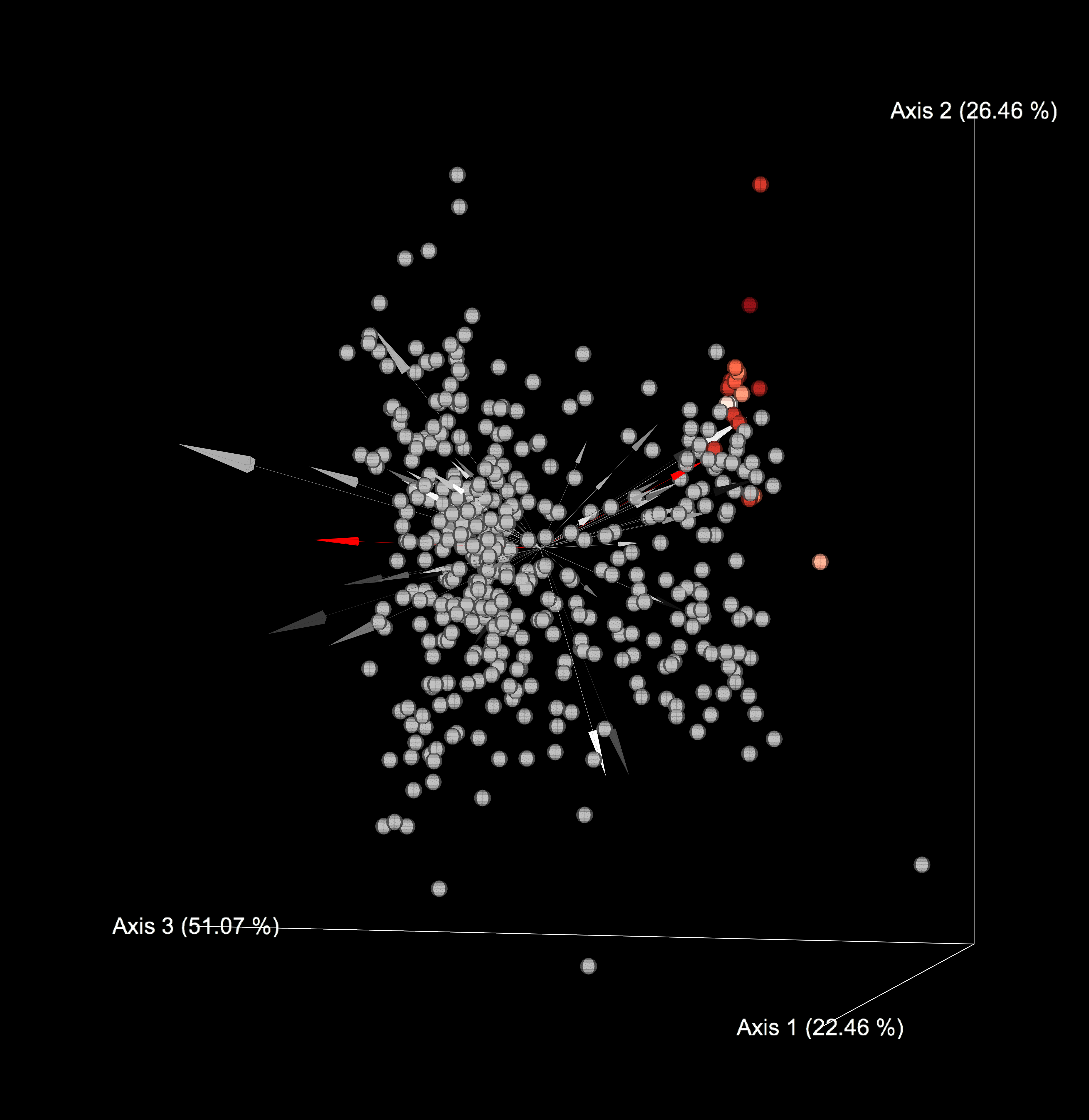
Here, the metabolite represent points and the arrows represent microbes. The points close together are indicative of metabolites that frequently co-occur with each other. Furthermore, arrows that have a small angle between them are indicative of microbes that co-occur with each other. Arrows that point in the same direction as the metabolites are indicative of microbe-metabolite co-occurrences. In the biplot above, the red arrows correspond to Pseudomonas aeruginosa, and the red points correspond to Rhamnolipids that are likely produced by Pseudomonas aeruginosa.
More information behind the parameters can found under qiime rhapsody --help
FAQs
Q: Looks like there are two different commands, a standalone script and a qiime2 interface. Which one should I use?!?
A: It'll depend on how deep in the weeds you'll want to get. For most intents and purposes, the qiime2 interface will more practical for most analyses. There are 3 major reasons why the standalone scripts are more preferable to the qiime2 interface, namely
-
Customized acceleration : If you want to bring down your runtime from a few days to a few hours, you may need to compile Tensorflow to handle hardware specific instructions (i.e. GPUs / SIMD instructions). It probably is possible to enable GPU compatiability within a conda environment with some effort, but since conda packages binaries, SIMD instructions will not work out of the box.
-
Checkpoints : If you are not sure how long your analysis should run, the standalone script can allow you record checkpoints, which can allow you to recover your model parameters. This enables you to investigate your model while the model is training.
-
More model parameters : The standalone script will return the bias parameters learned for each dataset (i.e. microbe and metabolite abundances). These are stored under the summary directory (specified by
--summary) under the namesembeddings.csv. This file will hold the coordinates for the microbes and metabolites, along with biases. There are 4 columns in this file, namelyfeature_id,axis,embed_typeandvalues.feature_idis the name of the feature, whether it be a microbe name or a metabolite feature id.axiscorresponds to the name of the axis, which either corresponds to a PC axis or bias.embed_typedenotes if the coordinate corresponds to a microbe or metabolite.valuesis the coordinate value for the givenaxis,embed_typeandfeature_id. This can be useful for accessing the raw parameters and building custom biplots / ranks visualizations - this also has the advantage of requiring much less memory to manipulate.
Q : You mentioned that you can use GPUs. How can you do that??
A : This can be done by running pip install tensorflow-gpu in your environment. See details here.
At the moment, these capabilities are only available for the standalone CLI due to complications of installation. See the --arm-the-gpu option in the standalone interface.
Q : Neural networks scare me - don't they overfit the crap out of your data?
A : Here, we are using shallow neural networks (so only two layers). This falls under the same regime as PCA and SVD. But just as you can overfit PCA/SVD, you can also overfit mmvec. Which is why we have Tensorboard enabled for diagnostics. You can visualize the cv_rmse to gauge if there is overfitting -- if your run is strictly decreasing, then that is a sign that you are probably not overfitting. But this is not necessarily indicative that you have reach the optimal -- you want to check to see if logloss has reached a plateau as shown above.
Q : I'm confused, what is Tensorboard?
A : Tensorboard is a diagnostic tool that runs in a web browser. To open tensorboard, make sure you’re in the rhapsody environment and cd into the folder you are running the script above from. Then run:
tensorboard --logdir .
Returning line will look something like:
TensorBoard 1.9.0 at http://Lisas-MacBook-Pro-2.local:6006 (Press CTRL+C to quit)
Open the website (highlighted in red) in a browser. (Hint; if that doesn’t work try putting only the port number (here it is 6006), adding localhost, localhost:6006). Leave this tab alone. Now any rhapsody output directories that you add to the folder that tensorflow is running in will be added to the webpage.
If working properly, it will look something like this
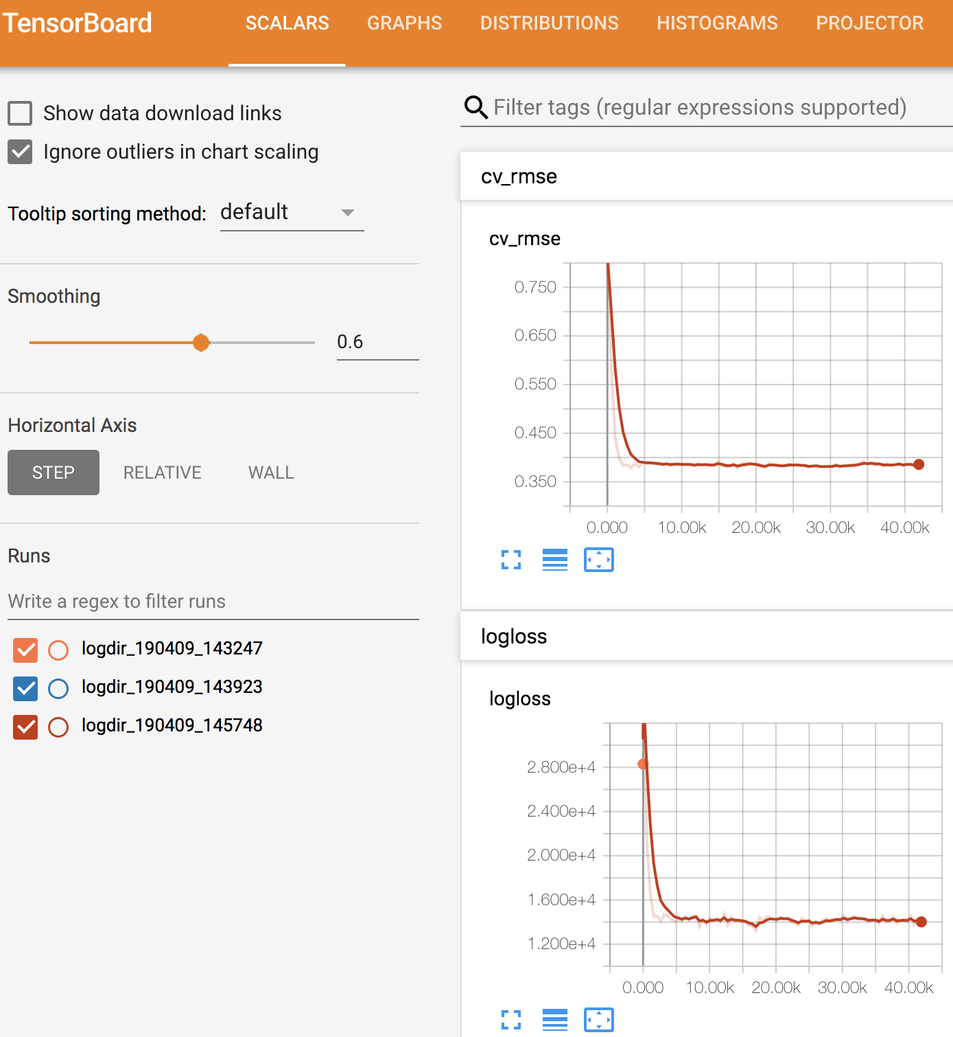
FIRST graph in Tensorflow; 'Prediction accuracy'. Labelled cv_rmse
This is a graph of the prediction accuracy of the model; the model will try to guess the metabolite intensitiy values for the testing samples that were set aside in the script above, using only the microbe counts in the testing samples. Then it looks at the real values and sees how close it was.
The second graph is the likelihood - if your likelihood values are plateaued, that is a sign that you have converged and reached at a local minima.
The x-axis is the number of iterations (meaning times the model is training across the entire dataset). Every time you iterate across the training samples, you also run the test samples and the averaged results are being plotted on the y-axis.
The y-axis is the average number of counts off for each feature. The model is predicting the sequence counts for each feature in the samples that were set aside for testing. So in the graph above it means that, on average, the model is off by ~0.75 intensity units, which is low. However, this is ABSOLUTE error not relative error (unfortunately we don't know how to compute relative errors because of the sparsity in these datasets).
You can also compare multiple runs with different parameters to see which run performed the best. If you are doing this, be sure to look at the training-column example make the testing samples consistent across runs.
Q : What's up with the --training-column argument?
A : That is used for cross-validation if you have a specific reproducibility question that you are interested in answering. It can also make it easier to compare cross validation results across runs. If this is specified, only samples labeled "Train" under this column will be used for building the model and samples labeled "Test" will be used for cross validation. In other words the model will attempt to predict the microbe abundances for the "Test" samples. The resulting prediction accuracy is used to evaluate the generalizability of the model in order to determine if the model is overfitting or not. If this argument is not specified, then 10 random samples will be chosen for the test dataset. If you want to specify more random samples to allocate for cross-validation, the num-random-test-examples argument can be specified.
Q : What sort of parameters should I focus on when picking a good model?
A : There are 3 different parameters to focus on, input-prior, output-prior and latent-dim
The --input-prior and --output-prior options specifies the width of the prior distribution of the coefficients, where the --input-prior is typically specific to microbes and the --output-prior is specific to metabolites.
For a prior of 1, this means 99% of entries in the embeddings (typically given in the U.txt and V.txt files are within -3 and +3 (log fold change). The higher differential-prior is, the more parameters can have bigger changes, so you want to keep this relatively small. If you see overfitting (accuracy and fit increasing over iterations in tensorboard) you may consider reducing the --input-prior and --output-prior in order to reduce the parameter space.
Another parameter worth thinking about is --latent-dim, which controls the number of dimensions used to approximate the conditional probability matrix. This also specifies the dimensions of the microbe/metabolite embeddings U.txt and V.txt. The more dimensions this has, the more accurate the embeddings can be -- but the higher the chance of overfitting there is. The rule of thumb to follow is in order to fit these models, you need at least 10 times as many samples as there are latent dimensions (this is following a similar rule of thumb for fitting straight lines). So if you have 100 samples, you should definitely not have a latent dimension of more than 10. Furthermore, you can still overfit certain microbes and metabolites. For example, you are fitting a model with those 100 samples and just 1 latent dimension, you can still easily overfit microbes and metabolites that appear in less than 10 samples -- so even fitting models with just 1 latent dimension will require some microbes and metabolites that appear in less than 10 samples to be filtered out.
Q : What does a good model fit look like??
A : Again the numbers vary greatly by dataset. But you want to see the both the logloss and cv_rmse curves decaying, and plateau as close to zero as possible.
Q : How long should I expect this program to run?
A : Both epochs and batch-size contribute to determining how long the algorithm will run, namely
Number of iterations = epoch # multiplied by the ( Total # of microbial reads / batch-size parameter)
This also depends on if your program will converge. The learning-rate specifies the resolution (smaller step size = smaller resolution, but may take longer to converge). You will need to consult with Tensorboard to make sure that your model fit is sane. See this paper for more details on gradient descent: https://arxiv.org/abs/1609.04747
If you are running this on a CPU, 16 cores, a run that reaches convergence should take about 1 day.
If you have a GPU - you maybe able to get this down to a few hours. However, some finetuning of the batch-size parameter maybe required -- instead of having a small batch-size < 100, you'll want to bump up the batch-size to between 1000 and 10000 to fully leverage the speedups available on the GPU.
Credits to Lisa Marotz (@lisa55asil), Yoshiki Vazquez-Baeza (@ElDeveloper) and Julia Gauglitz (@jgauglitz) for their README contributions.


Download files
Download the file for your platform. If you're not sure which to choose, learn more about installing packages.
Source Distribution
File details
Details for the file rhapsody-0.4.0.tar.gz.
File metadata
- Download URL: rhapsody-0.4.0.tar.gz
- Upload date:
- Size: 18.6 kB
- Tags: Source
- Uploaded using Trusted Publishing? No
- Uploaded via: twine/1.13.0 pkginfo/1.5.0.1 requests/2.21.0 setuptools/41.0.1 requests-toolbelt/0.9.1 tqdm/4.32.1 CPython/3.6.6
File hashes
| Algorithm | Hash digest | |
|---|---|---|
| SHA256 |
159cad70b5c34e9b36f24f8975933de06e541240151bd977be8c79ee609045b8
|
|
| MD5 |
4f3a0ff44823627ba9f4acdefc673302
|
|
| BLAKE2b-256 |
215b4dc0b411d571f5bb14c17d267de49631e6a2aaba63e3a9fbebddd094b0c8
|


