A simple python package for drawing attractive chemical reaction energy level diagrams.

Project description
rxnlvl
A simple python package for drawing attractive chemical reaction energy level diagrams.
What do I need?
rxnlvl requires Python 2.x or later.
###Install:
pip install rxnlvl
How do I work it?
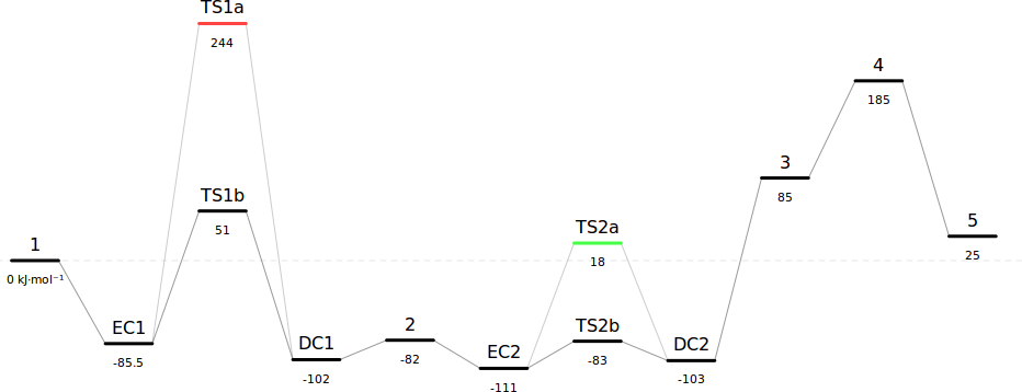
You can import the rxnlvl module to draw plots. A parser for those not versed in Python is planned, but even if you don't know python you should still be able to easily create plots. Here's the script that generates part of the image you see above (I truncated it for brevity but you can make plots as long as you want):
#! /usr/bin/python
from rxnlvl import *

# Plot
p = plot([25.0,10.0],vbuf=10.0,hbuf=5.0,bgcolour=None, qualified='sortof')

p +  level(energy(    0, 'kjmol'),  1,    '1',      0x0)
p +  level(energy(-85.5, 'kjmol'),  2,  'EC1',      0x0)
p +  level(energy(  244, 'kjmol'),  3, 'TS1a', 0xFF4444)
p +  level(energy(   51, 'kjmol'),  3, 'TS1b',      0x0)
p +  level(energy( -102, 'kjmol'),  4,  'DC1',      0x0)
p +  level(energy(  -82, 'kjmol'),  5,    '2',      0x0)

p +  edge(    '1',  'EC1', 0x0, 0.4, 'normal')
p +  edge(  'EC1', 'TS1a', 0x0, 0.2, 'normal')
p +  edge(  'EC1', 'TS1b', 0x0, 0.4, 'normal')
p +  edge( 'TS1a',  'DC1', 0x0, 0.2, 'normal')
p +  edge( 'TS1b',  'DC1', 0x0, 0.4, 'normal')
p +  edge(  'DC1',    '2', 0x0, 0.4, 'normal')


p + baseline(energy( 0.0, 'kjmol'),colour=0x0,mode='dashed',opacity=0.1)

p.write()
The boilerplate just tells Python where to find rxnlvl. Let's step through the rest:
###Plot creation:
p = plot([25.0,10.0],vbuf=10.0,hbuf=5.0,bgcolour=None, qualified='sortof')
The plot takes the following arguments:
dimensions- the width and height of the plot in cm.vbuf- the vertical margin as a percentage of the total height.hbuf- the horizontal margin as a percentage of the total height.bgcolour- the background colour of the image, as a 24-bit hexadecimal integer, orNone. IfNone, the background will be transparent!qualified- if True, the units in which each energy are specified will be pretty-printed in the image. If False, will only print the numeric values. If set to any string value, will only print units on the leftmost energy level, which is useful if you want to give units in your plot but don't want to clutter it up.
Now we can start adding elements to the plot.
###Time to add some levels:
p + level(energy( 0, 'kjmol'), 1, '1', 0x0)
Each level object takes the following arguments:
energy- anenergyobject which represents the relative energy of the level. Each energy has 2 arguments - the energy as a floating point number, and the units, which can be'kjmol','eh'(Hartrees),'ev'(electronvolts),'kcal'(thermochemical kilocalories per mole) or'wavenumber'.location- the ordinal location of the level in the scheme. This must be a positive nonzero integer. Different levels can share the same location.name- the name of the level in the scheme. Levels should not share the same name.colour- A 24-bit hexadecimal integer representing the colour of the level.
###Time to join the levels with edges:
p + edge( '1', 'EC1', 0x0, 0.4, 'normal')
Each edge object takes the folliwing arguments:
start- Thenameof the level that the edge originates from.end- Thenameof the level that the edge terminates at. This must be different tostart.colour- A 24-bit hexadecimal integer representing the colour of the edge.opacity- A float between 0.0 and 1.0 representing the opacity of the edge.mode- Choose either'normal'or'dashed'. Controls the appearance of the edge in terms of its dashed-linedness.
###Can we have a baseline ruled at 0.0 kJ/mol? Yes.
p + baseline(energy( 0.0, 'kjmol'),colour=0x0,mode='dashed',opacity=0.1)
You can have multiple baselines. The syntax should be fairly familiar:
energy- anenergyobject which represents the relative energy of the baseline. Each energy has 2 arguments - the energy as a floating point number, and the units, which can be'kjmol','eh'(Hartrees),'ev'(electronvolts),'kcal'(thermochemical kilocalories per mole) or'wavenumber'.colour- A 24-bit hexadecimal integer representing the colour of the edge.mode- Choose either'normal'or'dashed'. Controls the appearance of the edge in terms of its dashed-linedness.opacity- A float between 0.0 and 1.0 representing the opacity of the edge.
###Okay let's plot this.
svg = p.write()
with open('test.svg', 'w') as f:
    f.write(svg)
###Okay let's plot this with energy range
svg = p.write((-200,200))
with open('test.svg', 'w') as f:
    f.write(svg)
Will return *.svg file of your plot . Have fun!


Download files
Download the file for your platform. If you're not sure which to choose, learn more about installing packages.
Source Distribution
Built Distribution
Filter files by name, interpreter, ABI, and platform.
If you're not sure about the file name format, learn more about wheel file names.
Copy a direct link to the current filters
File details
Details for the file rxnlvl-0.3.10.tar.gz.
File metadata
- Download URL: rxnlvl-0.3.10.tar.gz
- Upload date:
- Size: 9.6 kB
- Tags: Source
- Uploaded using Trusted Publishing? No
- Uploaded via: twine/3.2.0 pkginfo/1.4.2 requests/2.23.0 setuptools/50.3.0 requests-toolbelt/0.8.0 tqdm/4.15.0 CPython/3.6.1
File hashes
| Algorithm | Hash digest | |
|---|---|---|
| SHA256 |
6f2adb998f76b42a1fd2df3444a0587481c988a508443bd822d84092e807c98f
|
|
| MD5 |
41541fe20d19cefcbf1e050108ac44da
|
|
| BLAKE2b-256 |
71e71fe897d093e1c3d98eda6d3d43d211aa13f954c27d4a2432ad9041325312
|
File details
Details for the file rxnlvl-0.3.10-py3-none-any.whl.
File metadata
- Download URL: rxnlvl-0.3.10-py3-none-any.whl
- Upload date:
- Size: 28.0 kB
- Tags: Python 3
- Uploaded using Trusted Publishing? No
- Uploaded via: twine/3.2.0 pkginfo/1.4.2 requests/2.23.0 setuptools/50.3.0 requests-toolbelt/0.8.0 tqdm/4.15.0 CPython/3.6.1
File hashes
| Algorithm | Hash digest | |
|---|---|---|
| SHA256 |
1c10bd8efae8c776e91923ab306074f2b4847f2abfcb304241d88600154018c7
|
|
| MD5 |
fbf0876f218727c98c0bea3b1a012099
|
|
| BLAKE2b-256 |
65a24d440266663dc6d665ac0e458a69ebf64692f1d6559ebf1ffb37db29c2b9
|


