Single-Cell Clustering Assessment Framework

Project description

SCCAF: Single Cell Clustering Assessment Framework
Single Cell Clustering Assessment Framework (SCCAF) is a novel method for automated identification of putative cell types from single cell RNA-seq (scRNA-seq) data. By iteratively applying clustering and a machine learning approach to gene expression profiles of a given set of cells, SCCAF simultaneously identifies distinct cell groups and a weighted list of feature genes for each group. The feature genes, which are overexpressed in the particular cell group, jointly discriminate the given cell group from other cells. Each such group of cells corresponds to a putative cell type or state, characterised by the feature genes as markers.
Requirements
This package requirements vary depending on the way that you want to install it (all three are independent, you don't need all these requirements):
- pip: if installation goes through pip, you will require Python3 and pip3 installed.
- Bioconda: if installation goes through Bioconda, you will require that conda is installed and configured to use bioconda channels.
- Docker container: to use SCCAF from its docker container you will need Docker installed.
- Source code: to use and install from the source code directly, you will need to have git, Python3 and pip.
The tool depends on other Python/conda packages, but these are automatically resolved by the different installation methods.
The tool has been tested with the following versions:
- conda: versions 4.7.5 and 4.7.10, but it should work with most other versions.
- Docker: version 18.09.2, but should work with most other versions.
- Python: versions 3.6.5 and 3.7. We don't expect this to work with Python 2.x.
- Pip3: version 9.0.3, but any version of pip3 should work.
This software doesn't require any non-standard hardware.
Installation
pip
You can install SCCAF with pip:
pip install sccaf
Installation time on laptop with 16 GB of RAM and academic (LAN) internet connection: <10 minutes.
Bioconda
You can install SCCAF with bioconda (please setup conda and the bioconda channel if you haven't first, as explained here):
conda install sccaf
Installation time on laptop with 16 GB of RAM and academic (LAN) internet connection: <5 minutes.
Available as a container
You can use the SCCAF tool already setup on a Docker container. You need to choose from the available tags here and replace it in the call below where it says <tag>.
docker pull quay.io/biocontainers/sccaf:<tag>
Note: Biocontainer's containers do not have a latest tag, as such a docker pull/run without defining the tag will fail. For instance, a valid call would be (for version 0.0.10):
docker run -it quay.io/biocontainers/sccaf:0.0.10--py_0
Inside the container, you can either use the Python interactive shell or the command line version (see below).
Installation (pull) time on laptop with 16 GB of RAM and academic (LAN) internet connection: ~10 minutes.
Use latest source code
Alternatively, for the latest version, clone this repo and go into its directory, then execute pip3 install .:
git clone https://github.com/SCCAF/sccaf
cd sccaf
# you might want to create a virtualenv for SCCAF before installing
pip3 install .
if your python environment is configured for python 3, then you should be able to replace python3 for just python (although pip3 needs to be kept). In time this will be simplified by a simple pip call.
Installation (pull) time on laptop with 16 GB of RAM and academic (LAN) internet connection: ~10 minutes.
Usage within Python environment
Use with pre-clustered anndata object in the SCANPY package
The main method of SCCAF can be applied directly to an anndata (AnnData is the main data format used by Scanpy) object in Python.
Before applying SCCAF, please make sure the doublets have been excluded and the batch effect has been effectively regressed.
Assessment of the quality of a clustering
Given a clustering stored in an anndata object adata under the key louvain, we would like to understand the quality (discrimination between clusters) with SCCAF:
from SCCAF import SCCAF_assessment, plot_roc
import scanpy as sc

adata = sc.read("path-to-clusterised-and-umapped-anndata-file")
y_prob, y_pred, y_test, clf, cvsm, acc = SCCAF_assessment(adata.X, adata.obs['louvain'], n=100)
returned accuracy is in the acc variable.
The ROC curve can be plotted:
import matplotlib.pyplot as plt

plot_roc(y_prob, y_test, clf, cvsm=cvsm, acc=acc)
plt.show()
Higher accuracy indicate better discrimination. And the ROC curve shows the problematic clusters.
Optimize an over-clustering
Given an over-clustered result, SCCAF optimize the clustering by merging the cell clusters that cannot be discriminated by machine learning.
Selecting the starting clustering
The selection of start clustering (or pre-clustering, which is an over-clustering) aims to find a clustering with only over-clustering but no under-clustering. To achieve this clustering, we suggest to combine well-established clustering (e.g., louvain clustering in SCANPY or K-means or SC3) with data visualization (tSNE). We can assume that all the discriminative cell clusters should be detectable in the tSNE plot. Then, we can find a clustering (e.g, louvain with a chosen resolution, 1.5 in the example case) that separates all the "cell islands" in the tSNE plot. To achieve a higher speed, we also suggest to have as few cell cluster as possible. For example, if both resolution 1.5 and resolution 2.0 do not include under-clustering, we suggest to use resolution 1.5 result as the start clustering.
# The batch effect MUST be regressed before applying SCCAF
adata = sc.read("path-to-clusterised-and-umapped-anndata-file")

# An initial over-clustering needs to be assigned in consistent with the prefix for the optimization.
# i.e., the optimization prefix is `L2`, the starting point of the optimization of `%s_Round0`%prefix, which is `L2_Round0`.

sc.tl.louvain(adata, resolution=1.5, key_added='L2_Round0')
# i.e., we aim to achieve an accuracy >90% for the whole dataset, optimize based on the PCA space:
SCCAF_optimize_all(ad=adata, plot=False, min_acc=0.9, prefix = 'L2', use='pca')
in the above run, all changes will be left on the adata anndata object and no plots
will be generated. If you want to see the plots (blocking the progress until you close them)
then remove the plots=False.
Within the anndata object, assignments of cells to clusters will be left in adata.obs['<prefix>_Round<roundNumber>'].
Notebook demo
You can find some demonstrative Jupyter Notebooks here:
- Zeisel Mouse Cortex Demo
- Expected execution time on a 16 GB RAM standard laptop: ~15 minutes
Usage from the command line
We have added convenience methods to use from the command line argument in the shell. This facilitate as well the inclusion in workflow systems.
Optimisation and general purpose usage
Given an annData dataset with louvain clustering pre-calculated (and batch corrected if needed):
sccaf -i <ann-data-input-file> --optimise --skip-assessment -s louvain -a 0.89 -c 8 --produce-rounds-summary
this will leave the result in new file named output.h5, which could be set via -o. In the current setting this will
produce a file named rounds.txt with the name of all optimisation rounds left in the output. This file
is used for later parallelisation (among different machines) of an assessment process to determine the step to choose
as final clustering.
To understand all options, simply execute sccaf --help.
Parallel run of assessments
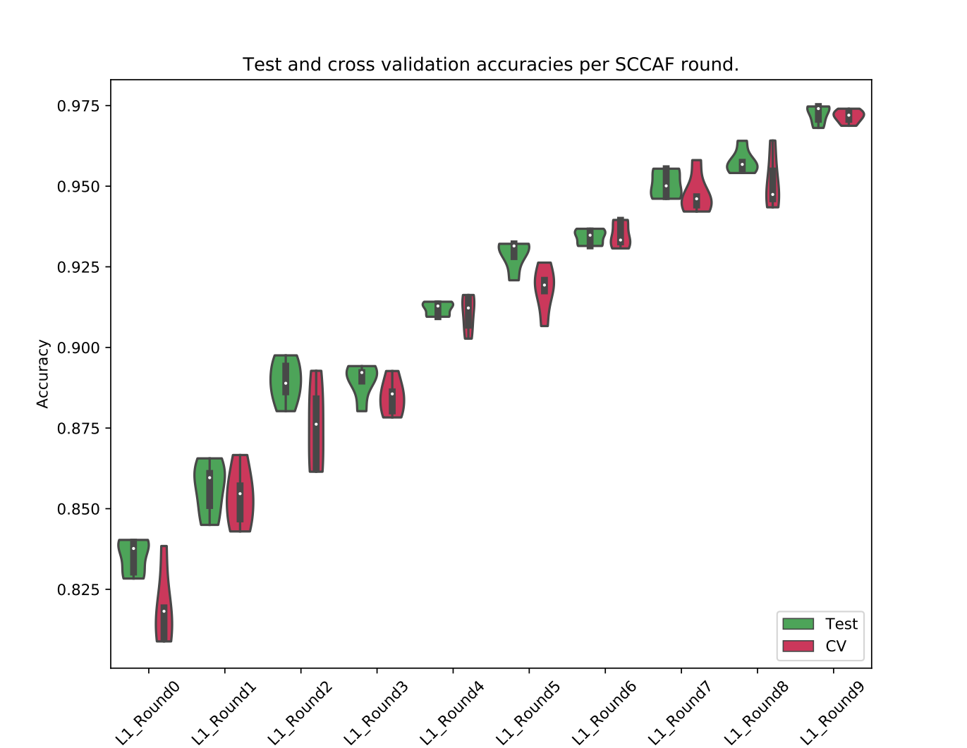
Once the optimisation has taken place, an strategy to choose the round to be used as final result is to observe the distribution of accuracies for each on multiple iterations of the assessment process. How the process is distributed is a matter of implementation of the local HPC or cloud system. Essentially, the process that can be repeated, per each round, is:
round=<name-of-the-round-in-the-output>
sccaf-asses -i output.h5 -o results/sccaf_assess_$round.txt --slot-for-existing-clustering $round --iterations 20 --cores 8
running the above for a number of different rounds will leave files in the results folder.
Merging parallel runs to produce plot
Once all assessment runs are done, the merging and plotting step can be run:
sccaf-assess-merger -i results -r rounds.txt -o rounds-acc-comparison-plot.png
This will produce a result like this:
Release history Release notifications | RSS feed


Download files
Download the file for your platform. If you're not sure which to choose, learn more about installing packages.
Source Distribution
Built Distribution
Filter files by name, interpreter, ABI, and platform.
If you're not sure about the file name format, learn more about wheel file names.
Copy a direct link to the current filters
File details
Details for the file SCCAF-0.0.10.tar.gz.
File metadata
- Download URL: SCCAF-0.0.10.tar.gz
- Upload date:
- Size: 1.7 MB
- Tags: Source
- Uploaded using Trusted Publishing? No
- Uploaded via: twine/3.1.1 pkginfo/1.5.0.1 requests/2.23.0 setuptools/46.1.3 requests-toolbelt/0.9.1 tqdm/4.45.0 CPython/3.6.7
File hashes
| Algorithm | Hash digest | |
|---|---|---|
| SHA256 |
9cfb215651cc4dfb0946294bdee568254f5b700f71c53e43018739dc9c7f18d4
|
|
| MD5 |
d20b42d8825934479dcadb4bdf627771
|
|
| BLAKE2b-256 |
47d0d7185c5d83baa68b781a44ba8b7c907c2e9b0ea2c950690bcd2a8446a4c2
|
File details
Details for the file SCCAF-0.0.10-py3-none-any.whl.
File metadata
- Download URL: SCCAF-0.0.10-py3-none-any.whl
- Upload date:
- Size: 27.4 kB
- Tags: Python 3
- Uploaded using Trusted Publishing? No
- Uploaded via: twine/3.1.1 pkginfo/1.5.0.1 requests/2.23.0 setuptools/46.1.3 requests-toolbelt/0.9.1 tqdm/4.45.0 CPython/3.6.7
File hashes
| Algorithm | Hash digest | |
|---|---|---|
| SHA256 |
4cfff1a1c303097cc309d6b448ace79eff98f97d288097d91e71a1820244838d
|
|
| MD5 |
1c441470389e95537b4ab0566c116b78
|
|
| BLAKE2b-256 |
db90f617a7ce7971137257925dcd92ae1a6a4633b9aa0c3a3955fb8e965d7092
|


