
scikit-opt


Swarm Intelligence in Python
(Genetic Algorithm, Particle Swarm Optimization, Simulated Annealing, Ant Colony Algorithm, Immune Algorithm,Artificial Fish Swarm Algorithm in Python)
- Documentation: https://scikit-opt.github.io/scikit-opt/#/en/
- 文档: https://scikit-opt.github.io/scikit-opt/#/zh/
- Source code: https://github.com/guofei9987/scikit-opt
- Help us improve scikit-opt https://www.wjx.cn/jq/50964691.aspx
install
pip install scikit-opt
For the current developer version:
git clone git@github.com:guofei9987/scikit-opt.git
cd scikit-opt
pip install .
Features
Feature1: UDF
UDF (user defined function) is available now!
For example, you just worked out a new type of selection function.
Now, your selection function is like this:
-> Demo code: examples/demo_ga_udf.py#s1
# step1: define your own operator:
def selection_tournament(algorithm, tourn_size):
    FitV = algorithm.FitV
    sel_index = []
    for i in range(algorithm.size_pop):
        aspirants_index = np.random.choice(range(algorithm.size_pop), size=tourn_size)
        sel_index.append(max(aspirants_index, key=lambda i: FitV[i]))
    algorithm.Chrom = algorithm.Chrom[sel_index, :]  # next generation
    return algorithm.Chrom
Import and build ga
-> Demo code: examples/demo_ga_udf.py#s2
import numpy as np
from sko.GA import GA, GA_TSP

demo_func = lambda x: x[0] ** 2 + (x[1] - 0.05) ** 2 + (x[2] - 0.5) ** 2
ga = GA(func=demo_func, n_dim=3, size_pop=100, max_iter=500, lb=[-1, -10, -5], ub=[2, 10, 2],
        precision=[1e-7, 1e-7, 1])
Regist your udf to GA
-> Demo code: examples/demo_ga_udf.py#s3
ga.register(operator_name='selection', operator=selection_tournament, tourn_size=3)
scikit-opt also provide some operators
-> Demo code: examples/demo_ga_udf.py#s4
from sko.operators import ranking, selection, crossover, mutation

ga.register(operator_name='ranking', operator=ranking.ranking). \
    register(operator_name='crossover', operator=crossover.crossover_2point). \
    register(operator_name='mutation', operator=mutation.mutation)
Now do GA as usual
-> Demo code: examples/demo_ga_udf.py#s5
best_x, best_y = ga.run()
print('best_x:', best_x, '\n', 'best_y:', best_y)
Until Now, the udf surport
crossover,mutation,selection,rankingof GA scikit-opt provide a dozen of operators, see here
For advanced users:
-> Demo code: examples/demo_ga_udf.py#s6
class MyGA(GA):
    def selection(self, tourn_size=3):
        FitV = self.FitV
        sel_index = []
        for i in range(self.size_pop):
            aspirants_index = np.random.choice(range(self.size_pop), size=tourn_size)
            sel_index.append(max(aspirants_index, key=lambda i: FitV[i]))
        self.Chrom = self.Chrom[sel_index, :]  # next generation
        return self.Chrom

    ranking = ranking.ranking


demo_func = lambda x: x[0] ** 2 + (x[1] - 0.05) ** 2 + (x[2] - 0.5) ** 2
my_ga = MyGA(func=demo_func, n_dim=3, size_pop=100, max_iter=500, lb=[-1, -10, -5], ub=[2, 10, 2],
        precision=[1e-7, 1e-7, 1])
best_x, best_y = my_ga.run()
print('best_x:', best_x, '\n', 'best_y:', best_y)
feature2: GPU computation
We are developing GPU computation, which will be stable on version 1.0.0
An example is already available: https://github.com/guofei9987/scikit-opt/blob/master/examples/demo_ga_gpu.py
feature3: continue to run
(New in version 0.3.6)
Run an algorithm for 10 iterations, and then run another 20 iterations base on the 10 iterations before:
from sko.GA import GA

func = lambda x: x[0] ** 2
ga = GA(func=func, n_dim=1)
ga.run(10)
ga.run(20)
Quick start
1. Differential Evolution
Step1:define your problem
-> Demo code: examples/demo_de.py#s1
'''
min f(x1, x2, x3) = x1^2 + x2^2 + x3^2
s.t.
    x1*x2 >= 1
    x1*x2 <= 5
    x2 + x3 = 1
    0 <= x1, x2, x3 <= 5
'''


def obj_func(p):
    x1, x2, x3 = p
    return x1 ** 2 + x2 ** 2 + x3 ** 2


constraint_eq = [
    lambda x: 1 - x[1] - x[2]
]

constraint_ueq = [
    lambda x: 1 - x[0] * x[1],
    lambda x: x[0] * x[1] - 5
]
Step2: do Differential Evolution
-> Demo code: examples/demo_de.py#s2
from sko.DE import DE

de = DE(func=obj_func, n_dim=3, size_pop=50, max_iter=800, lb=[0, 0, 0], ub=[5, 5, 5],
        constraint_eq=constraint_eq, constraint_ueq=constraint_ueq)

best_x, best_y = de.run()
print('best_x:', best_x, '\n', 'best_y:', best_y)
2. Genetic Algorithm
Step1:define your problem
-> Demo code: examples/demo_ga.py#s1
import numpy as np


def schaffer(p):
    '''
    This function has plenty of local minimum, with strong shocks
    global minimum at (0,0) with value 0
    '''
    x1, x2 = p
    x = np.square(x1) + np.square(x2)
    return 0.5 + (np.sin(x) - 0.5) / np.square(1 + 0.001 * x)
Step2: do Genetic Algorithm
-> Demo code: examples/demo_ga.py#s2
from sko.GA import GA

ga = GA(func=schaffer, n_dim=2, size_pop=50, max_iter=800, lb=[-1, -1], ub=[1, 1], precision=1e-7)
best_x, best_y = ga.run()
print('best_x:', best_x, '\n', 'best_y:', best_y)
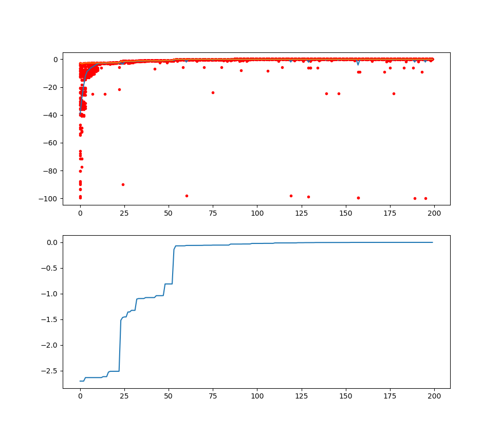
Step3: plot the result
-> Demo code: examples/demo_ga.py#s3
import pandas as pd
import matplotlib.pyplot as plt

Y_history = pd.DataFrame(ga.all_history_Y)
fig, ax = plt.subplots(2, 1)
ax[0].plot(Y_history.index, Y_history.values, '.', color='red')
Y_history.min(axis=1).cummin().plot(kind='line')
plt.show()
2.2 Genetic Algorithm for TSP(Travelling Salesman Problem)
Just import the GA_TSP, it overloads the crossover, mutation to solve the TSP
Step1: define your problem. Prepare your points coordinate and the distance matrix.
Here I generate the data randomly as a demo:
-> Demo code: examples/demo_ga_tsp.py#s1
import numpy as np
from scipy import spatial
import matplotlib.pyplot as plt

num_points = 50

points_coordinate = np.random.rand(num_points, 2)  # generate coordinate of points
distance_matrix = spatial.distance.cdist(points_coordinate, points_coordinate, metric='euclidean')


def cal_total_distance(routine):
    '''The objective function. input routine, return total distance.
    cal_total_distance(np.arange(num_points))
    '''
    num_points, = routine.shape
    return sum([distance_matrix[routine[i % num_points], routine[(i + 1) % num_points]] for i in range(num_points)])
Step2: do GA
-> Demo code: examples/demo_ga_tsp.py#s2
from sko.GA import GA_TSP

ga_tsp = GA_TSP(func=cal_total_distance, n_dim=num_points, size_pop=50, max_iter=500, prob_mut=1)
best_points, best_distance = ga_tsp.run()
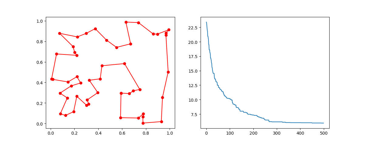
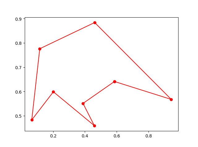
Step3: Plot the result:
-> Demo code: examples/demo_ga_tsp.py#s3
fig, ax = plt.subplots(1, 2)
best_points_ = np.concatenate([best_points, [best_points[0]]])
best_points_coordinate = points_coordinate[best_points_, :]
ax[0].plot(best_points_coordinate[:, 0], best_points_coordinate[:, 1], 'o-r')
ax[1].plot(ga_tsp.generation_best_Y)
plt.show()
3. PSO(Particle swarm optimization)
3.1 PSO with constraint
Step1: define your problem:
-> Demo code: examples/demo_pso.py#s1
def demo_func(x):
    x1, x2, x3 = x
    return x1 ** 2 + (x2 - 0.05) ** 2 + x3 ** 2
Step2: do PSO
-> Demo code: examples/demo_pso.py#s2
from sko.PSO import PSO

pso = PSO(func=demo_func, dim=3, pop=40, max_iter=150, lb=[0, -1, 0.5], ub=[1, 1, 1], w=0.8, c1=0.5, c2=0.5)
pso.run()
print('best_x is ', pso.gbest_x, 'best_y is', pso.gbest_y)
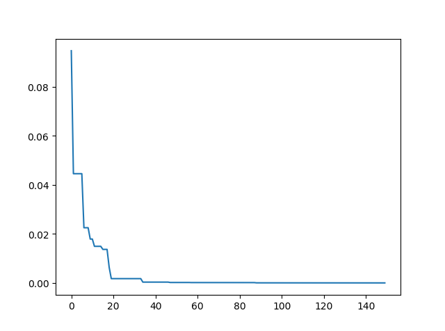
Step3: Plot the result
-> Demo code: examples/demo_pso.py#s3
import matplotlib.pyplot as plt

plt.plot(pso.gbest_y_hist)
plt.show()
3.2 PSO without constraint
-> Demo code: examples/demo_pso.py#s4
pso = PSO(func=demo_func, dim=3)
fitness = pso.run()
print('best_x is ', pso.gbest_x, 'best_y is', pso.gbest_y)
4. SA(Simulated Annealing)
4.1 SA for multiple function
Step1: define your problem
-> Demo code: examples/demo_sa.py#s1
demo_func = lambda x: x[0] ** 2 + (x[1] - 0.05) ** 2 + x[2] ** 2
Step2: do SA
-> Demo code: examples/demo_sa.py#s2
from sko.SA import SA

sa = SA(func=demo_func, x0=[1, 1, 1], T_max=1, T_min=1e-9, L=300, max_stay_counter=150)
best_x, best_y = sa.run()
print('best_x:', best_x, 'best_y', best_y)
Step3: Plot the result
-> Demo code: examples/demo_sa.py#s3
import matplotlib.pyplot as plt
import pandas as pd

plt.plot(pd.DataFrame(sa.best_y_history).cummin(axis=0))
plt.show()
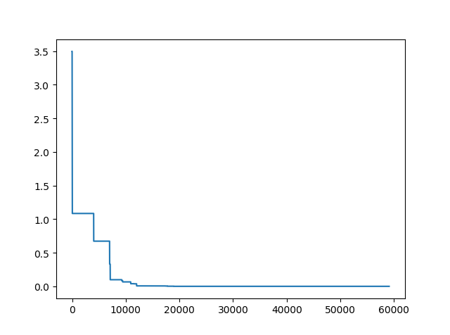
Moreover, scikit-opt provide 3 types of Simulated Annealing: Fast, Boltzmann, Cauchy. See more sa
4.2 SA for TSP
Step1: oh, yes, define your problems. To boring to copy this step.
Step2: DO SA for TSP
-> Demo code: examples/demo_sa_tsp.py#s2
from sko.SA import SA_TSP

sa_tsp = SA_TSP(func=cal_total_distance, x0=range(num_points), T_max=100, T_min=1, L=10 * num_points)

best_points, best_distance = sa_tsp.run()
print(best_points, best_distance, cal_total_distance(best_points))
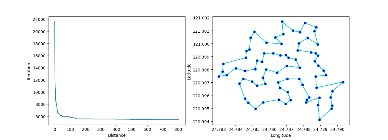
Step3: plot the result
-> Demo code: examples/demo_sa_tsp.py#s3
from matplotlib.ticker import FormatStrFormatter

fig, ax = plt.subplots(1, 2)

best_points_ = np.concatenate([best_points, [best_points[0]]])
best_points_coordinate = points_coordinate[best_points_, :]
ax[0].plot(sa_tsp.best_y_history)
ax[0].set_xlabel("Iteration")
ax[0].set_ylabel("Distance")
ax[1].plot(best_points_coordinate[:, 0], best_points_coordinate[:, 1],
           marker='o', markerfacecolor='b', color='c', linestyle='-')
ax[1].xaxis.set_major_formatter(FormatStrFormatter('%.3f'))
ax[1].yaxis.set_major_formatter(FormatStrFormatter('%.3f'))
ax[1].set_xlabel("Longitude")
ax[1].set_ylabel("Latitude")
plt.show()
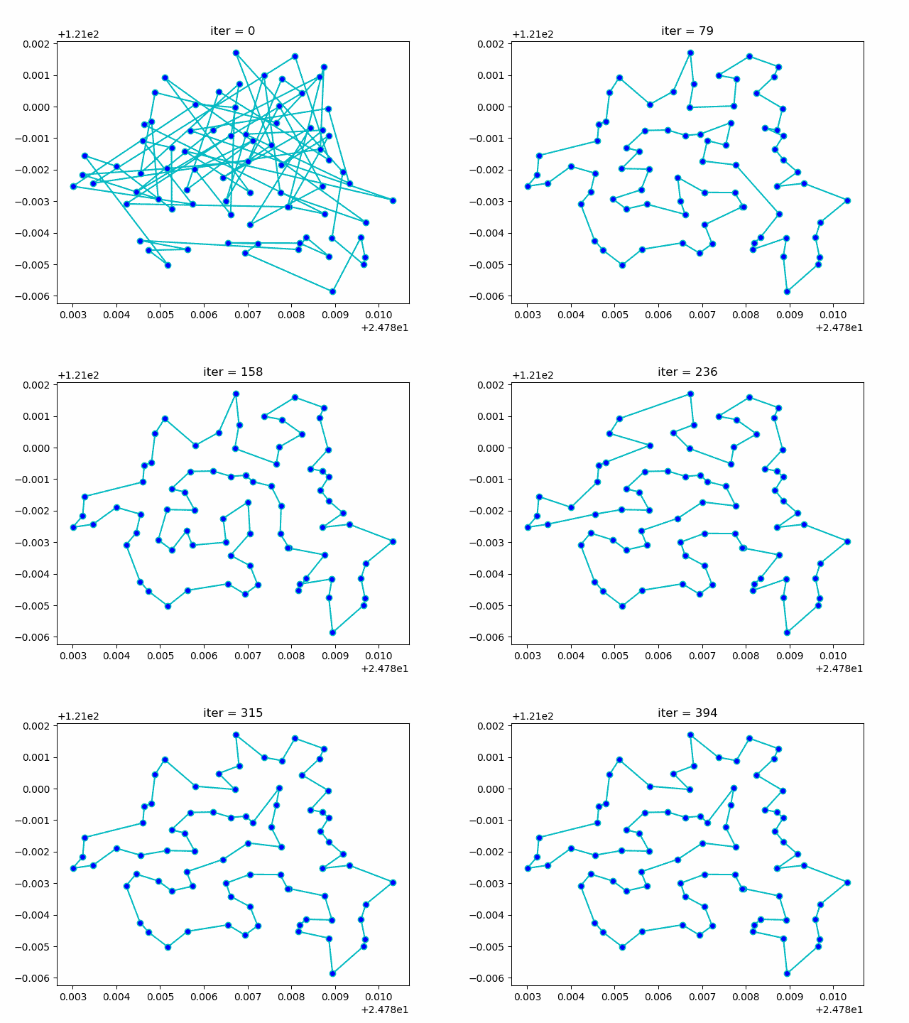
More: Plot the animation:
5. ACA (Ant Colony Algorithm) for tsp
-> Demo code: examples/demo_aca_tsp.py#s2
from sko.ACA import ACA_TSP

aca = ACA_TSP(func=cal_total_distance, n_dim=num_points,
              size_pop=50, max_iter=200,
              distance_matrix=distance_matrix)

best_x, best_y = aca.run()
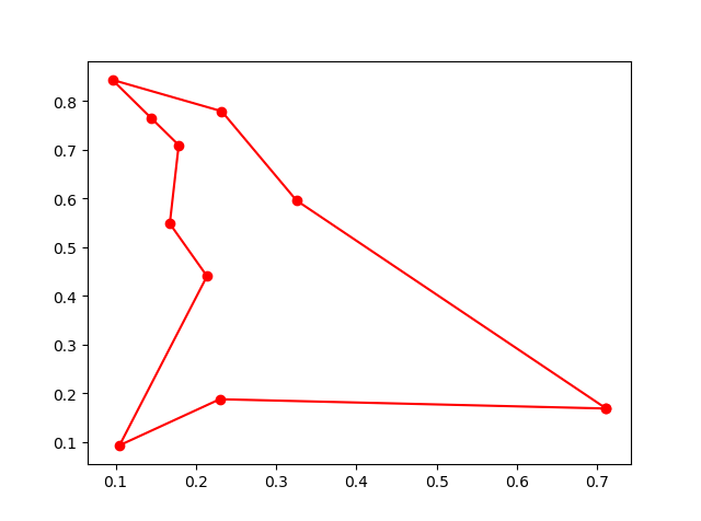
6. immune algorithm (IA)
-> Demo code: examples/demo_ia.py#s2
from sko.IA import IA_TSP

ia_tsp = IA_TSP(func=cal_total_distance, n_dim=num_points, size_pop=500, max_iter=800, prob_mut=0.2,
                T=0.7, alpha=0.95)
best_points, best_distance = ia_tsp.run()
print('best routine:', best_points, 'best_distance:', best_distance)
7. Artificial Fish Swarm Algorithm (AFSA)
-> Demo code: examples/demo_afsa.py#s1
def func(x):
    x1, x2 = x
    return 1 / x1 ** 2 + x1 ** 2 + 1 / x2 ** 2 + x2 ** 2


from sko.AFSA import AFSA

afsa = AFSA(func, n_dim=2, size_pop=50, max_iter=300,
            max_try_num=100, step=0.5, visual=0.3,
            q=0.98, delta=0.5)
best_x, best_y = afsa.run()
print(best_x, best_y)
1 maintainer

Metadata
1 maintainer
Release files for scikit-opt 0.5.6
For a detailed explanation of source distributions (sdists) and built distributions (wheels), please see the package formats documentation.
Source distribution (sdist)
| File | Size | Uploaded | Provenance | Actions |
|---|---|---|---|---|
| scikit-opt-0.5.6.tar.gz | 22.0 kB | Without provenance | Details for scikit-opt-0.5.6.tar.gz |
Built distribution (wheel)
| File | Interpreter | ABI | Platform | Actions Reset |
|---|---|---|---|---|
| scikit_opt-0.5.6-py3-none-any.whl | Python 3 | none | any | Details for scikit_opt-0.5.6-py3-none-any.whl |
Total release size: 49.1 kB
Release files / scikit-opt-0.5.6.tar.gz
| Download URL | scikit-opt-0.5.6.tar.gz |
|---|---|
| Size | 22.0 kB |
| Tags | Source |
|
SHA-256 checksum How to use checksums |
288dd1c4e27be972dbaa2f63ff04025461c7cee71466aeaec57caf7620bb61c9
|
|
BLAKE2b-256 checksum How to use checksums |
0ff3a5e631a84f63800f0a04a03bbedeae3e612ed54821d34947c9d2ba4697bc
|
| Upload date | |
|
Uploaded using Trusted Publishing? What is trusted publishing? |
No |
| Uploaded via |
twine/3.1.1 pkginfo/1.5.0.1 requests/2.22.0 setuptools/46.1.3 requests-toolbelt/0.9.1 tqdm/4.42.1 CPython/3.7.6
|
Release files / scikit_opt-0.5.6-py3-none-any.whl
| Download URL | scikit_opt-0.5.6-py3-none-any.whl |
|---|---|
| Size | 27.0 kB |
| Tags | Python 3 |
|
SHA-256 checksum How to use checksums |
2d02558c5a0e5d1bb148490bfbca1a458fb56772c60246e9355f820a6be0fdac
|
|
BLAKE2b-256 checksum How to use checksums |
d57b0dd4d95e82749ede54654f5b802014b283a479c1161b828552a46a3c2572
|
| Upload date | |
|
Uploaded using Trusted Publishing? What is trusted publishing? |
No |
| Uploaded via |
twine/3.1.1 pkginfo/1.5.0.1 requests/2.22.0 setuptools/46.1.3 requests-toolbelt/0.9.1 tqdm/4.42.1 CPython/3.7.6
|
Security for scikit-opt 0.5.6
Provenance
Provenance describes where a file came from. On PyPI, provenance is shared via attestations, which provide a verifiable record of the build or publishing details. View details, limitations and caveats.
No provenance found
None of the files in this release were uploaded with provenance metadata.
A note on package security
PyPI is a repository for distributing packages, not a service for auditing them. While third-party security researchers and our staff do their best to detect and remove malicious packages, PyPI cannot guarantee the quality, security or suitability of any given package.
To learn more about protecting yourself from malicious actors, visit our package security documentation.














