Estimate IV- and PV-curves given photovoltaic cell datasheet parameters.

Project description
solarcell
Estimate IV- and PV-curves given photovoltaic cell datasheet parameters. Capable of generating combined curves for solar arrays with temperature and light intensity gradients. Assumes ideal bypass and blocking diodes for all cells.
Available for download on PyPI.
pip install solarcell
Usage
See the examples contained within this repository. Please also consider reading the related blog post, "How To Estimate Complex Solar Array Power Curves".
import numpy as np
from matplotlib import pyplot as plt
from solarcell import solarcell
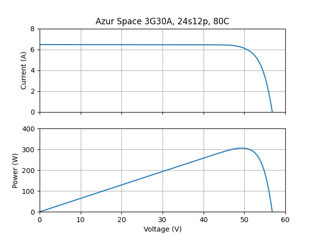
# Azur Space 3G30A triple-junction solar cells in a 24s12p configuration.
# Isc/Imp are specified in (A, A/C), Voc/Vmp are specified in (V, V/C).
# Temperature is specified in C. Intensity is unitless and scales Isc/Imp.
azur3g30a = solarcell(
isc=(0.5196, 0.00036), # short-circuit current, temp coefficient
voc=(2.690, -0.0062), # open-circuit voltage, temp coefficient
imp=(0.5029, 0.00024), # max-power current, temp coefficient
vmp=(2.409, -0.0067), # max-power voltage, temp coefficient
area=30.18, # solar cell area in square centimeters
t=28, # temperature at which the above parameters are specified
)
array = azur3g30a.array(t=np.full((24, 12), 80), g=np.ones((24, 12)))
print(array)
# Isc = 6.460 A, Voc = 56.82 V
# Imp = 6.201 A, Vmp = 49.33 V, Pmp = 305.9 W
fig, (ax0, ax1) = plt.subplots(nrows=2, sharex=True)
v = np.linspace(0, array.voc, 1000)
ax0.plot(v, array.iv(v)), ax0.grid()
ax1.plot(v, array.pv(v)), ax1.grid()
Background
A numeric optimization procedure is used to best fit the classic photovoltaic cell single diode model equation to the datasheet parameters at the reference temperature. Curves at other temperatures are derived relative to this initial curve fit by way of a linear transformation (plus a sigmoid smoothing function) that maintains the characteristic shape of the curve. Combining cells in series/parallel with different IV-curves is done by linear interpolation.
When computing a curve, the provided temperatures and intensities are generally organized as follows: cell(t, g) accepts single values, string(t, g) accepts one-dimensional arrays, and array(t, g) accepts two-dimensional arrays (where strings make up the columns). A cache is implemented to increase speed for repeated computations; rounding by the user will yield better performance.
References
- Amit Jain, Avinashi Kapoor, Exact analytical solutions of the parameters of real solar cells using Lambert W-function, Solar Energy Materials and Solar Cells, Volume 81, Issue 2, 2004, Pages 269-277, ISSN 0927-0248, https://doi.org/10.1016/j.solmat.2003.11.018.
Release history Release notifications | RSS feed


Download files
Download the file for your platform. If you're not sure which to choose, learn more about installing packages.
Source Distribution
Built Distribution
Filter files by name, interpreter, ABI, and platform.
If you're not sure about the file name format, learn more about wheel file names.
Copy a direct link to the current filters
File details
Details for the file solarcell-0.2.0.tar.gz.
File metadata
- Download URL: solarcell-0.2.0.tar.gz
- Upload date:
- Size: 6.2 kB
- Tags: Source
- Uploaded using Trusted Publishing? No
- Uploaded via: poetry/1.4.1 CPython/3.11.0 Windows/10
File hashes
| Algorithm | Hash digest | |
|---|---|---|
| SHA256 |
386fb69514905951ef17cdf1b55abc359c5f530d34b66c1eb702ee8eec819e17
|
|
| MD5 |
ceb29f1e349c41cf57d5c530bfcf9e6f
|
|
| BLAKE2b-256 |
acb8a250f591a0facc888fdf0b50ddc0a4bcd91c7484de881625eb03108366e1
|
File details
Details for the file solarcell-0.2.0-py3-none-any.whl.
File metadata
- Download URL: solarcell-0.2.0-py3-none-any.whl
- Upload date:
- Size: 6.7 kB
- Tags: Python 3
- Uploaded using Trusted Publishing? No
- Uploaded via: poetry/1.4.1 CPython/3.11.0 Windows/10
File hashes
| Algorithm | Hash digest | |
|---|---|---|
| SHA256 |
24d592964f75c0ed3f0a583aaf77f9c9723d7bf89bbc98a0d4de98de5d9cc06e
|
|
| MD5 |
6653d82e78a7882dae598cac3f102e38
|
|
| BLAKE2b-256 |
734996e9cb2175d70f002523cada4f55f359216d79142bf11c18954afc3feff7
|


